In this study, a novel damage detection framework for skeletal structures is presented. The introduced scheme is based on the optimization-based model updating method. A new multipopulation framework, namely, the Famine Algorithm, is introduced that hopes to reduce the number of objective function evaluations needed. Furthermore, using static displacement patterns, a damage-sensitive feature named pseudo-kinetic energy is presented. By exploiting the new feature, an efficient cost function is developed. Two mathematical benchmark problems and a two-membered truss for damage detection problem are depicted in 2D space to track the search behavior of the Famine Algorithm and show the changes in the search space when using the new feature. Four numerical examples, including three trusses and a frame structure, are used to evaluate the overall performance of the proposed damage detection methods. Moreover, an experimental shear frame is studied to test the performance of the suggested method in real-life problems. The obtained results of the examples reveal that the proposed method can identify and quantify the damaged elements accurately by only utilizing the first five vibrating modes, even in noise-contaminated conditions.

1. Introduction

The structural health monitoring (SHM) field continues to grow due to its importance for structural safety and preventing catastrophic events, such as the sudden collapse of buildings, bridges, and other significant structures. Because of the inefficiency of dated methods like visual inspection in the early detection of damage, methods based on processing the data measured by sensors were introduced. Due to the reduction of computational costs in recent decades, a more detailed analysis of vibration data is available to detect damage. A detailed explanation of early developments in damage detection can be found in [1, 2]. The dynamic characteristics of a structure are sensitive to changes in its physical properties. When the damage causes a change, it is possible to find its severity and location by solving the inverse dynamic problem. There are several tools to solve this problem.

Recently, novel tools, especially artificial intelligence, including optimization algorithms and machine learning, have become increasingly popular because of their advances. These tools have made significant developments in the field of health monitoring. High-speed Internet and cloud computing have made these tools easier to implement in real-life structures [3]. First-order Eigen perturbation (FOP) techniques have emerged as a fast and efficient method for continuous monitoring of the structures. They will detect changes in the dynamic characteristics of the structure with minimum computation needed [4, 5]. As a result of these advancements, monitoring important yet complex infrastructures such as wind turbines is now easier than before [6]. A comprehensive survey of recent advances in the field can be found in [7].

One of the favored methods for damage detection in the literature is the optimization-based model updating method. Because of the ill-posed conditions of the damage detection problem, especially in complex structures and large finite element models, a robust and efficient optimization algorithm is needed. Metaheuristic optimization algorithms are easy to implement in any optimization problem and do not require complex calculations essential to classic mathematical methods. Therefore, they are a popular choice for a range of engineering problems. Numerous studies have been carried out using this framework. For example, Kaveh et al. [8] used plasma generation optimization developed in [9] with a hybrid objective function to locate damage in skeletal structures. Ghannadi and Kourehli [10] investigated the performance of the multiverse optimizer developed by Mirjalili et al. [11] in SHM. Ghahremani et al. [12] used the covariance matrix adaptation optimization algorithm (CMA-ES) introduced in [13] to solve the damage detection inverse problem. Zare Hosseinzadeh et al. [14] used the cuckoo search algorithm presented in [15] with a flexibility-based objective function to locate damage when there is a limited number of sensors. Dinh-Cong et al. [16] investigated the damage detection of the plate-like structures with modal strain energy change as the objective function and the Jaya algorithm by the author in [17] for optimization. Kaveh et al. introduced an innovative method in [18] that by changing the boundaries of the problem in the first phase of damage detection, the search by shuffled shepherd optimization algorithm [19] became more robust. Aval and Mohebian developed an improved version of the biology migration algorithm to minimize an objective function that takes the combined joint and member damage into account.

As for the versatility of metaheuristic algorithms, most of the optimization algorithms mentioned above have been utilized in multiple fields. For instance, numerous examples can be found in structural design problems like weight and geometry optimization. Gandomi et al. [20] used cuckoo search algorithm with Lévy flights in 13 well-known design problems. Kaveh et al. [21] improved the Jaya algorithm with a multipopulation scheme and reported its performance in the discrete variable structural optimization problem. The plasma generation optimization algorithm’s performance was initially tested with constrained weight optimization problems [9]. Cantero-Chinchilla et al. developed a robust optimal sensor configuration by utilizing the CMA-ES optimization algorithm [22]. A more comprehensive description of metaheuristics can be found in Kaveh and Bakhshpoori’s book [23].

One of the tools to improve the search process of metaheuristic algorithms is to break the population into multiple subpopulations. Partitioning technics or multipopulation technics were used since the beginning of metaheuristic algorithms. For instance in genetic algorithm [24], the migration or Island model [25] was introduced in which the population is broken into multiple subpopulations and each subpopulation will begin to evolve independently, and eventually, the migration will take place between them. The dynamic subswarm number strategy was proposed in [26] for the PSO algorithm. In this scheme, as the search progresses, the number of subpopulations and subsequently the number of their members will gradually change from multiple subpopulations with two members to one population with all the members. Blackwell proposed a method in which the number of subpopulations can change. In this method, namely, the self-adaptive multipopulation technique [27], the search will begin with one population. When the members in this population seem to have converged, another random population will get added to the search until the maximum number of subpopulations is reached. Consequently, the worst subpopulation will get removed, so another random one can be added. Several other methods use clustering techniques, such as K-means, to group members together and form subpopulations based on their distance from each other [28–31]. A more detailed survey on different multipopulation methods can be found in [32, 33].

Due to its high accuracy and efficiency, in this study, the damage localization problem is solved with the optimization-based model updating method. Optimization-based model updating has two main components: the optimization algorithm and the objective function, which will locate the damages when it is minimized. The goal is to minimize the differences between the damaged structure and the predicted finite element model. Hence, when the objective function, formulated from damage-sensitive features, reaches its minimum value, it can be stated that the differences are minimized and the updated model is a good representative of the conditions in the damaged structure. Improvements in the optimization algorithm and the objective function should be regarded to improve the damage detection process discussed in this study. In complex structures, the analysis will require more time and resources, and reducing even a small portion of the analysis time will result in considerable cost savings.

Hence, firstly, a novel multipopulation scheme named the Famine Algorithm is introduced, which will help the search find the result in fewer analyses or reach higher accuracy at the same number of structural analyses. Secondly, a new damage-sensitive feature named pseudo-kinetic energy is suggested, and by utilizing this feature, an objective function is defined. The proposed objective function expands the feature for each member and mode shape to carry out as detailed comparison between models as possible.

The rest of this study is structured as follows. In Section 2, the Famine Algorithm is introduced. In Section 3, damage detection methodology, including the feature and objective function definition, is presented. Section 4 is dedicated to evaluating the performance of the suggested methods. Finally, in Section 5, the conclusions are discussed.

2. Famine Algorithm

In times of Famine, resources become scarce, and deciding how to allocate them properly becomes paramount. Assuming that several groups are tasked with searching for new resources, two questions come to mind: How should these search agents be grouped, and What is the optimal way to distribute resources between them so that as many discoveries as possible can be made with the least number of resources consumed? Similarly, the resource in optimization problems is the analysis time or the number of function evaluations (NFE), and the agents are the optimization algorithm’s search agents. Because of the high cost of analysis, especially when the problem is in high dimensions and complex, the reasonable analysis time is limited. Hence, the proposed optimization scheme is based on the indication that the resources available are scarce and costly, and therefore, their usage should be planned so that the maximum possible result can be gained with as little analysis time as possible.

2.1. Search Agent Grouping

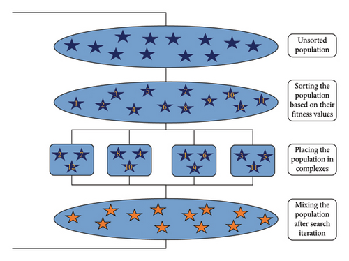
The groups created must be in a way that they can equally represent the whole population, and no weak or overly strong groups must be created. Weak-membered groups will potentially waste resources, and overly strong groups will lead to early convergence. Shuffled complex evolution [34] was proposed as a multipopulation scheme that uses partitioning and regrouping search agents based on their fitness values for better dispersion of members in each subpopulation. In this technique, the population is sorted based on its members’ fitness values. Subsequently, if there are m subpopulations (C₁, C₂, …, C_m), the first m best members of the population (x₁, x₂, …, x_m) will be selected and placed inside the complexes and the process will continue until all the populations are placed, so every complex has a member of the best, moderate, and weak portion of the population. Complexes will start to evolve independently from each other, and after the search phase, the population is regrouped, mixed, and sorted to be partitioned again. This cycle will continue until the end criteria are met. This partitioning and regrouping will act as a global search mechanism that gathers new and different agents in the complexes at each turn, so information between search agents from different parts of the search space gets shared. Because the members change at each turn, the chances of early convergence and stagnation in complexes are low. This technique was utilized in various metaheuristics, including frog leaping algorithm, bat algorithm, shuffled shepherd, and shuffled Jaya algorithms [18, 21, 35–37]. However, in this method, the first complex will get the best members of each sorted piece, and again, it will not meet our goal of creating an equal representation of the whole population. This problem can be solved by randomizing the assignment of each piece of the sorted population to complexes. Hence, every complex has a random member from each piece, and there is no order to its selection [21]. The schematic of the described process, named random shuffle complex grouping (RSCG), can be seen in Figure 1, and this method is utilized in this study.

Details are in the caption following the image — **Figure 1**
Open in figure viewer PowerPoint

Schematic of random shuffle complex grouping.

2.2. Resource Allocation

After dividing the population into groups, the main question remains: How should scarce resources be divided? The group expected to perform better than others should have a higher chance of getting more resources. The mean objective function values (MOFV) of members in each group could indicate their capabilities in the upcoming search. Thus, the group with a lower MOFV is expected to perform better.

2.2.1. Rank-Based Fitness Assignment

To calculate the probability of selection for groups, a fitness function is utilized to assign each group a fitness value. The groups are sorted from highest MOFV to lowest, and based on their new position, a fitness value, FitnV, is assigned to each of them according to the following:

()

where NG is the number of groups, and pos indicates the position of each group in the sorted order. The X refers to the root of the polynomial equation (2) that could be either linear or nonlinear [38]; however, the nonlinear format, due to not having zero probability in the worst position, appeared to perform better in this study. SP is selection pressure with values between [1, NG − 2] for the nonlinear form.

2.2.2. Roulette Wheel Selection

The resource allocation can be carried out by having the probability of selection P(x_i). One of the most popular probabilistic selection methods, used frequently in optimization algorithms, especially genetic algorithm [39, 40], is roulette wheel selection. Based on their fitness values, the groups will occupy a specific wheel slice, and selection can occur by turning the wheel and checking the location of the pointer when it stops (see Figure 2(a)). Another way to model this process is by calculating the cumulative probabilities of selection (or fitness values) and generating a random number between 0 and the maximum of the cumulative probabilities of selection using uniform distribution to see where the random number is placed on the wheel. The probability of selection for each group can be calculated as

()

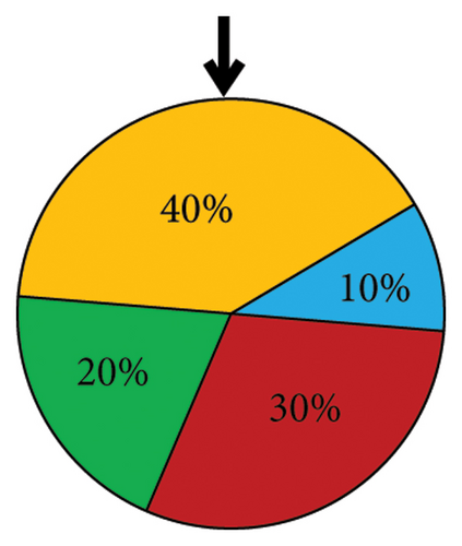
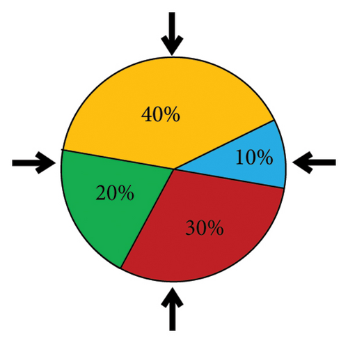
When one of the groups is significantly better than the others, it will occupy most of the wheel. Therefore, when selection occurs multiple times, the least probable choices may be ignored entirely. The stochastic universal sampling (SUS) method was introduced to solve this issue [39]. Multiple equally spaced pointers are implemented in this method instead of one pointer, and the turning occurs once (see Figure 2(b)). Therefore, the issue of selection bias is not present anymore. This study utilized the SUS method for its better overall performance.

2.3. Search Strategy

The Famine Algorithm is a multipopulation scheme, and a search algorithm is still needed to complete the optimization process. Like many other multipopulation techniques, the Famine Algorithm is easily compatible with any population-based metaheuristics, and there is a wide variety of selections for choosing. The Teaching-Learning-Based Optimization (TLBO) algorithm [41] was chosen for this study. Having a satisfactory performance coupled with being straightforward to code and implement and having a minimum need for search parameter adjustments were some of the reasons for choosing this search algorithm.

2.3.1. Teaching-Learning-Based Optimization Algorithm

As the name suggests, the interactions happening in a school class are the inspiration for this algorithm. The overall process consists of two phases. The first phase, named the teaching phase, uses the best solution found so far as the teacher and tries to update the positions of the rest of the students, so the average score of the class is improved toward the teacher’s score according to the following equations:

()

where DM_i (difference mean) is the step that the i^th member takes to reach its new position X_new,i from its old position X_old,i and r_i is a randomly generated number between [0, 1]. The learning capabilities of students vary from one to another; therefore, for modeling this effect, a random teaching factor T_F is implemented that could be 1 or 2. M_i refers to the current mean of the population’s positions and M_new is the new desirable mean of positions that should be the position of the teacher.

The second phase of the algorithm models the interaction between students trying to learn from each other and is called the learning phase. Each student will randomly get grouped with another member of the population and try to learn from them. If the chosen teammate has a better position, the student will try to get closer to it. Conversely, if the student’s position is better than their teammate’s, he or she will go in the opposite direction. These movements are implemented by

()

in which X_i and X_j are the students’ positions and

is a random vector generated between [0, 1]. In both steps, if the newfound position is better than the previous one, it will get accepted; otherwise, the position will not change [41].

2.4. Steps of the Famine Algorithm

By implementing the mechanisms defined above, the steps of the Famine Algorithm can be described as follows. First, an initial population with Nind agents is randomly created in the feasible search space and their objective function values are calculated, so they can be sorted considering their fitness. The sorted population is then divided into NG groups using the RSCG process so that every group has equally good, moderate, and weak members of the population. For each group, the MOFV is calculated. Using the fitness function, MOFVs are turned into fitness values, so resource allocation can occur. By utilizing the SUS method, the search turns are divided between groups so that the best-performing group has a higher chance of searching. It is worth mentioning that in each turn, NG resources are available, and by performing probabilistic sortation, multiple groups may not get the chance to search, and conversely, some groups with better previous performance will search multiple times. After getting the resources, the groups will start to search by employing the functions of the TLBO algorithm accordingly. Furthermore, the newfound positions will get updated, and all members will gather together to get sorted and grouped again. This process will continue until the ending criteria are met. The described process can be seen in Figure 3.

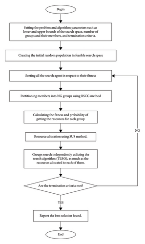
By distributing the resources as stated above, two main benefits are gained. First of all, if the population is on the verge of converging to the global optima or there are no local optima traps nearby, there is no need for all of the population to search the space, and the best-performing group can use more resources to advance the population further much more quickly. Secondly, if there are local minima traps nearby, and the leading groups get trapped, the members of groups that did not have the chance to get the resources to search will remain outside of the trap. Hence, in the next turn, when the population is mixed together and regrouped, a few members in each group remain outside and have a chance of getting the rest of the group out of the trap. As a result, resource usage has been optimized, and the risk of early convergence has been reduced.

3. Damage Detection Methodology

This section presents the needed formulations for modeling the inverse damage detection problem, including damage formulation, noise effect modeling, and objective function definition.

3.1. Damage Formulation

Damage occurrence in a structure will reduce the damaged element’s stiffness. The cause of this change can be traced to a reduction in cross-sectional area, modulus of elasticity, or moment of inertia. Assuming changes in modulus of elasticity, the global stiffness matrix in the damaged state, K^d, can be calculated as

()

where k_j is the elemental stiffness matrix, nelem is the total number of elements, and α_j is the damage ratio. The damage ratio, as a difference between the modulus of elasticity of the damaged (

) and healthy (

) elements, is described as

()

The damage ratio can vary in the range of [0, 1], where 0 denotes a healthy element and 1 indicates total loss of stiffness.

3.2. Noise Effect

In real-life applications, data obtained from sensors are polluted with noise that cannot be removed entirely and will later show its effect in obtained modal data. Hence, in numerical simulations, this phenomenon should be taken into consideration. There is no need to derive the modal data from the polluted acceleration data because the utilized feature does not contain the acceleration data. Therefore, the preferred method in the literature is to pollute the modal data directly [42]. For this purpose, the following equations are used:

()

where

and

are i^th obtained natural frequencies after and before noise pollution, respectively. Similarly,

and

are i^th obtained vibrational mode shapes after and before noise pollution, respectively, and

indicates the largest absolute value in i^th mode shape vector. N_ω and N_φ are noise levels selected for natural frequency and mode shapes. Moreover, r_ω and r_φ are randomly generated numbers and vectors with zero mean and unity variance that follow the Gaussian distribution.

3.3. Objective Function

The free vibration equation can be expressed as

()

where K and M are the global stiffness and mass matrixes of the finite element model. Moreover, ω_i and φ_i are the i^th natural frequency and mode shape vector, respectively, and ndo f is the number of degrees of freedom.

3.3.1. Modal Kinetic Energy

The modal kinetic energy of the structure was introduced as a damage-sensitive feature in [43] and has been broadly utilized in damage detection and model updating studies [42]. The formulation of this feature can be expressed as

()

where MKE_ij is the corresponding modal kinetic energy of the i^th eigenvalue and j^th element with a mass matrix of M_j. The corresponding objective function (E) using the modal kinetic energy change ratio can be defined as

()

where

and

are the elemental modal kinetic energy of the i^th eigenvalues and j^th element for the actual existing and guessed analytical structures, respectively.

3.3.2. Pseudo-Kinetic Energy

The displacement of structure nodes under static loads can be calculated using the flexibility matrix. As Hooke’s law states, static displacement matrix S has a linear relationship with flexibility matrix G and force matrix F, as shown in the following equation:

()

Therefore, each column of the flexibility matrix represents the static displacement pattern of every degree of freedom when a unit load is applied to its corresponding degree of freedom. For example, the first column of flexibility shows the static displacements of the structure when unit force is placed on the structures’ first degree of freedom. It is possible to approximate the flexibility matrix using several first-mode shapes and natural frequencies [14, 44]. Hence, the flexibility matrix G_i derived from i^th modal properties can be calculated as

()

where nm refers to the total number of modes used. The static displacement pattern ({S_ri}) of all degrees of freedom corresponding to the flexibility matrix derived from i^th mode shape and unit force on the r^th degree of freedom is calculated using (15). Therefore, the j^th element’s pseudo-kinetic energy (PKE_rji), derived from i^th eigenvalue and the r^th statistical displacement pattern, can be expressed as

()

By considering one mode shape to calculate the flexibility matrix and placing unit force on each degree of freedom, ndof static displacement vectors can be calculated. As a result, instead of one kinetic energy value for each member, there are ndof × ndof pseudo-kinetic energy values available. Therefore, there is ndof² times more detailed data available to compare and locate the damaged elements. The locality of this method will be beneficial in the case of minor damages that are not discernible in changes of more global features.

3.3.3. Proposed Objective Function

The primary objective function used in this study will compare the PKE_i matrix, that its members are derived from i^th modal data, by calculating the change ratio of the largest eigenvalue (Maxeigen) of the PKE_i matrix using the norm function in MATLAB as

()

In this equation,

and

are the pseudo-kinetic energy matrixes of the existing damaged structure and guessed analytical model derived from the i^th modal data, and | | yields absolute values. By using the procedure introduced above, the modal data are expanded into multiple statistical patterns representing various loading conditions and mode shape patterns. Moreover, the data are compared at the lowest level before summation so every minor change of statistical patterns due to damage is accounted for in calculations. To define the optimization problem, the damage detection formulation can be summarized as follows:

()

3.3.4. Error Calculation

To calculate the accuracy of the damage detection process, an error index (EI) is defined as

()

where

and

are the actual existing and identified damage ratios of j^th element, respectively.

3.4. Illustrated Comparison of the Objective Functions

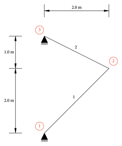
To illustrate the changes that happened to search space when using the introduced novel feature PKE and objective function (F), a two-bar truss structure is defined and modeled, as seen in Figure 4. The simple truss is comprised of two members with a modulus of elasticity and a material density of 200 GPa and 7780 kg/m³, respectively. The cross-sectional area of members is 0.001 m². The two variable damage inverse problem is modeled with 20% and 35% reductions of stiffness in members 1 and 2, respectively. The two-dimensional search space of the objective function for conventional MKE change ratio (E) and the novel introduced objective function (F) is shown in Figure 5. To better show the details of the search spaces, the vertical axes are depicted in logarithmic scale. Moreover, to solve the plotting problem of the minus infinity value of log (f = 0) in the global minimum, a small constant (ε) equal to 1.0–⁶ is added to all the objective function values (log (f + ε)).

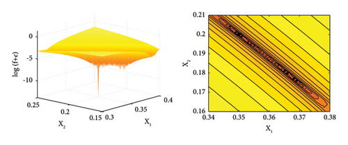
As seen in Figure 5(a), in the search space relating to the conventional MKE change ratio, there are multiple local minima that can hinder the search process by trapping the search agents. In contrast, after exploiting the static displacement to calculate PKE and objective function (F), it seems the search space shown in Figure 5(b) has been cleared of local minima, leaving only the global minimum. This change will simplify the search space and increase the overall convergence speed by removing the local minima traps.

4. Method Efficiency Evaluation

4.1. Performance Monitoring and Convergence Behavior

To better understand the difference that the Famine Algorithm makes on the base optimization algorithm’s performance, the positions of the search agents and their behavior are studied in this section. Mathematical benchmark problems are one of the primal methods of studying the performance of optimization problems. Therefore, one unimodal and one multimodal mathematical benchmark problem, along with the 2-bar truss damage detection problem in Sections 3 and 4, are selected and investigated in 2D space. Furthermore, details and the formulation for these mathematical benchmark problems can be seen in Table 1 and Figure 6.

Table 1. Description of mathematical benchmark problems.

Function	Range	f_min
	[−100, 100]	0
	[−50, 50]	0

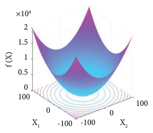
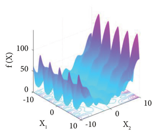
In Figures 7–9, the search process of both Famine and base TLBO algorithms are depicted for the f₁, f₂, and 2-bar truss damage detection problems, respectively. The dots in the search space represent the ten best search agents of algorithms in noted iterations. Moreover, the positions in the initial population, first iteration, 10^th iteration, and 20^th iteration are included to show the progress thoroughly. Incepting the results in Figures 7–9, it is apparent that the convergence speed of the Famine Algorithm exceeds the base TLBO algorithm. In all three cases, in the 10^th and 20^th iterations, the Famine Algorithm seems to have converged to the global minimum, whereas the TLBO algorithm’s members are still dispersed, and in the case of the f₂ function, which has multiple local minima traps, some of its members seem to have gotten trapped.

4.2. Numerical Examples

In this section, numerical examples of damage detection problems have been investigated. Four structures are modeled, including two- and three-dimensional trusses and a planner frame. Apart from ideal noise-free conditions, noise pollution effects are also studied in all of the examples. Since the mode shapes are generally measured less accurately than natural frequencies, the natural frequency and mode shape data are perturbed by 1% and 3% noises, respectively [18, 45–47]. Furthermore, for taking the incomplete data effects into account, only the first five natural frequencies and their corresponding mode shapes are used in all numerical examples. To have an unbiased and statically valid comparison, all of the reported results are average values of 30 independent runs for each case.

4.2.1. 25-Bar Planar Truss

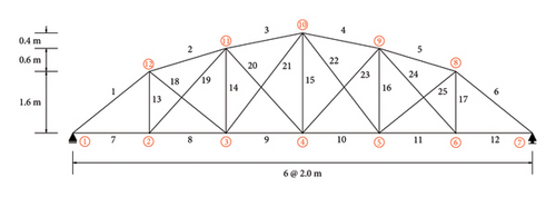
The first numerical example is the 25-bar planner truss, which can be seen in Figure 10. Properties of the elements constructing this model are modulus of elasticity (E) of 200 GPa and material density (ρ) equal to 7780 kg/m³, and all members have 10 cm² of cross-sectional area (A). This structure has 12 nodes and three constraints resulting in 21 degrees of freedom. Three different damage scenarios, including single, double, and multiple damaged elements, are considered, which can be seen in Table 2, and the only first five mode shapes and natural frequencies are used. To demonstrate the difference in performance between the conventional MKE and the newly introduced PKE features, objective functions F and E are both used to determine damage location and severity. Moreover, three well-known features, including modified total modal assurance criterion (MTMAC) [10, 48], modal strain energy-based index (MSEBI) [49], and multiple damage location assurance criterion (MDLAC) [50], are tested for better comparison of the error index and performance of the suggested method. The details of these additional features and their respective objective functions can be found in Table 3. Apart from the objective functions, all other search conditions are similar. The Famine Algorithm is used to find the minima, and five groups of four search agents are allocated for the task. The maximum NFE is set to 10000.

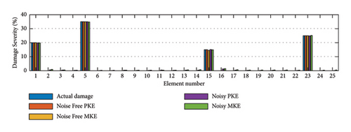
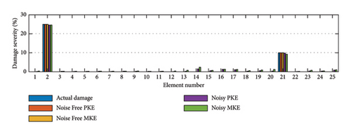
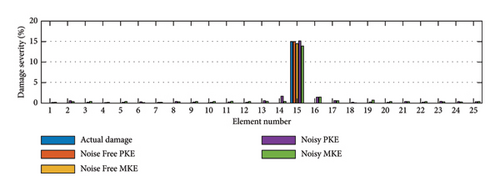
Table 2. Damage scenarios considered for the 25-bar planar truss.

Scenario	I				II		III
Element number	1	5	15	23	2	21	15
Damage ratio (%)	20	35	15	25	25	10	15

Table 3. Description of the additional objective functions and their features.

Feature	Objective function


∆F = (ω^h−ω^e)/ω^h δF(α) = (ω^h−ω^a)/ω^h	F_MDLAC = −MDLAC

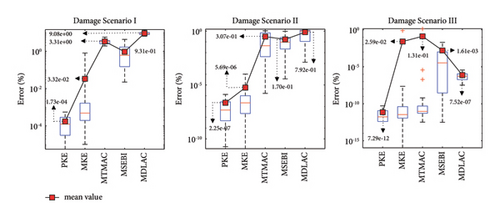
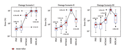
Figure 11 shows the average results obtained from the PKE and MKE functions in noisy and noise-free states. As evident in Figure 11, the Famine Algorithm successfully found the minima of both objective functions and location, and the severity of damages is discernible, though minor errors can be spotted. To further show the differences in damage detection of objective functions, the error indexes are depicted with box plots for all scenarios in Figure 12. As can be seen in all scenarios, the novel PKE feature and objective function (F) have performed better, considering all objective functions were given the same number of NFEs. The mean values of EI are smaller for the PKE in all cases, and the noise-free damage scenario III has the most significant difference of 3.55 × 10⁹ times smaller EI in PKE than in base MKE. The error present in noisy conditions is considerably more prominent than in noise-free runs that are rooted in noise contamination. However, the PKE has been more successful in ignoring these effects than other objective functions. Moreover, the negative effects of incomplete modal data are more prominent in some features. It can be interpreted that expanding each mode shape into statistical displacement in each member and degree of freedom has helped PKE to significantly ignore these errors. However, using some features together has proven to help their accuracy, but PKE on its own by simplifying the search space has shown better convergence. Particularly, in noisy conditions when convergence becomes challenging, certain features encountered difficulties in converging within the limited NFE available. This challenge is reflected by the observed EI values.

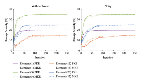
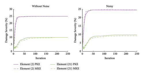
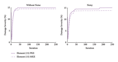
To better see the search progression that resulted in these outcomes, the convergence histories of damage values for damaged elements are shown in Figure 13. Considering the much fewer local minima traps in the objective function (F), it is not surprising that in most cases, damage values converged faster for PKE rather than MKE. In damage scenario III, the superior performance of the PKE feature is more evident as more accurate and faster convergence can be seen.

4.2.2. 25-Bar Spatial Truss

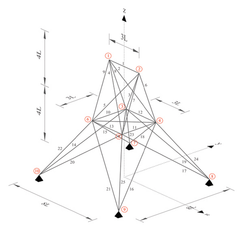
The second structure selected in this study is the three-dimensional 25-bar truss structure, as shown in Figure 14. Elements of this truss have a modulus of elasticity of 10⁴ ksi and material density of 0.1 lbm/in³, and cross-sectional area of 10 in². This example has ten nodes, and six of them are free. Each free node has three degrees of freedom, resulting in 18 degrees of freedom for the whole structure. Again, only the first five mode shapes are considered in this example. The damage cases employed are shown in Table 4. Both single and multiple damage scenarios are considered.

Table 4. Damage scenarios considered for the 25-bar spatial truss.

Scenario	I			II
Element number	5	13	22	13
Damage ratio (%)	20	25	20	20

In this example, the efficiency of the proposed novel optimization scheme is compared against multiple well-known optimization algorithms, including TLBO, Gray Wolf Optimization (GWO), and PSO algorithms.

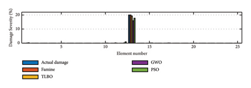
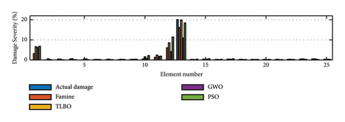
25 search agents that are divided into five groups for Famine Algorithm are assigned to the optimization algorithms, and 30000 NFEs are given to them to search the feasible area of the inverse problem. The GWO algorithm is coded according to [51], and for PSO algorithm, the embedded MATLAB toolbox is used. A summary of the used parameters of these algorithms is listed in Table 5. The damage detection results for mentioned algorithms are presented in Figure 15. The Famine Algorithm and TLBO seem to have performed better than their competitors. To better understand the results, the EI values are presented in Table 6. The EI values seem to validate the previous claim. In all the scenarios, the Famine Algorithm has the smallest EI values compared to the other three, especially in noise-free conditions.

Table 5. Parameters of Famine, TLBO, GWO, and PSO algorithms for 25-bar spatial truss structure.

Algorithm name	Famine	TLBO	GWO	PSO
Number of iterations	600	600	1200	1200
Population size	25	25	25	25

Table 6. Statistical error index results for the 25-bar spatial truss.

Scenario		I		II
Noise condition	Optimization algorithm	EI		EI
Noise condition	Optimization algorithm	Ave	Std	Ave	Std
Noise-free	Famine	5.28E − 05	9.47E − 05	2.50E − 08	7.35E − 08
	TLBO	6.22E − 03	1.04E − 02	2.85E − 02	1.56E − 01
	GWO	1.54E + 00	9.53E − 01	1.98E − 01	3.42E − 01
	PSO	1.39E + 00	2.90E + 00	1.51E − 01	3.58E − 01

Noisy	Famine	1.03E + 00	4.82E − 01	1.13E + 00	6.68E − 01
	TLBO	1.59E + 00	9.51E − 01	1.60E + 00	1.00E + 00
	GWO	2.34E + 00	9.64E − 01	1.21E + 00	6.73E − 01
	PSO	2.06E + 00	2.21E + 00	1.56E + 00	1.06E + 00

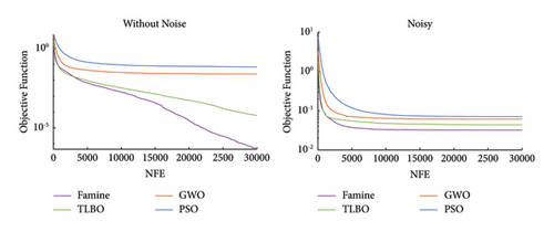
The reason for the Famine Algorithm’s superiority can be realized by investigating the convergence histories. Figure 16 shows that in all the attempts, the Famine Algorithm has the quickest convergence, and in three of four conditions, it was able to find smaller minima than its counterparts due to its better use of the NFEs and the avoidance of local minima. TLBO, GWO, and PSO algorithms are placed above the Famine Algorithms, respectively, and some premature convergences have occurred because of the local minima traps. The best performance of Famine Algorithm can be seen in noise-free conditions of scenario II because there is no noise error to hinder the search and force convergence. As a result, the Famine Algorithm was able to find the damage 1.14 × 10⁶, 7.92 × 10⁶, and 6.04 × 10⁶ times more accurately than TLBO, GWO, and PSO algorithms, respectively.

4.2.3. 23-Element Asymmetrical Planar Frame

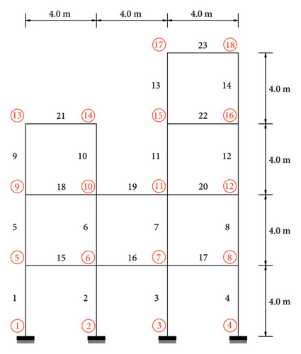
The third employed example is an asymmetrical planner frame with 23 elements [18]. The details of the constructed model can be seen in Figure 17. The figure shows that the frame is constructed of 14 columns and nine beams connected in 14 free nodes of 18 total nodes. Each free node having three degrees of freedom will result in the 42 total degrees of freedom for the structure. The material density and modulus of elasticity for all the elements are ρ = 7850 kg/m³ and E = 200 GPa, respectively. However, the cross-sectional area, moment of inertia, and mass per unit length for beam and column elements differ. For column elements, A_column = 1.6 × 10⁻² m², I_column = 3.5 × 10⁻⁴ m⁴, and = 125.6 kg/m, respectively. Moreover, for beam elements, A_beam = 1.62 × 10⁻² m², I_beam = 3.85 × 10⁻⁴ m⁴, and = 1300 kg/m, respectively. Both multiple and single damage cases are considered, and the details are given in Table 7. It is worth mentioning that like before in this example, only the first five mode shapes are used.

Table 7. Damage scenarios considered for the 23-element asymmetrical planar frame.

Scenario	I			II
Element number	4	18	21	10
Damage ratio (%)	15	35	20	25

The Famine Algorithm and base TLBO algorithm were utilized to minimize the objective function (F) to study the performance of the damage detection process suggested by this study in frame structures. The search conditions for both algorithms are considered the same, so the maximum number of NFE is set to 40000 to ensure convergence, and the total search agent’s numbers are set to 32 that are grouped in three eight-membered groups for the Famine Algorithm.

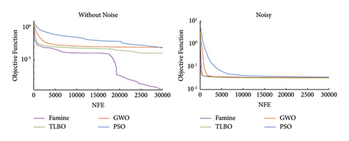
Figure 18 shows the damage detection results for both algorithms in noisy and noise-free conditions. To further clarify the differences in the performance of these two algorithms, the convergence histories are plotted in Figure 19. In all cases, it is evident that the Famine Algorithm has a quicker convergence rate than the basic TLBO algorithm. Therefore, given a specific objective function value, the Famine Algorithm will be able to reach that value using fewer NFEs than the TLBO algorithm.

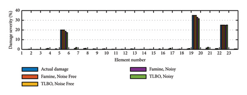
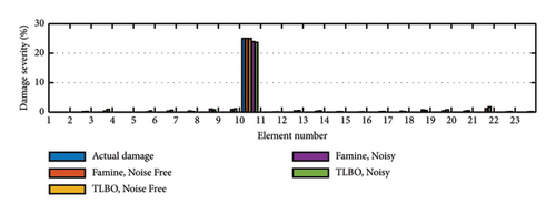
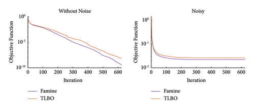
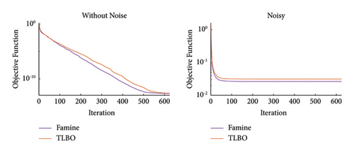
As for the performance of the objective function, the statistical results for EI values are presented in Table 8 that show ignorable error percentages attesting to its efficient accuracy. In addition, the EI values in cases that use the Famine Algorithm are lower, resulting from quicker convergence and smaller objective function values found. The most considerable difference can be seen in the noise-free damage scenario (I), with 32.9 times more accurate results in the Famine Algorithm.

Table 8. Statistical EI results of the 23-element asymmetrical planar frame.

Scenario		I		II
Noise condition	Optimization algorithm	EI		EI
Noise condition	Optimization algorithm	Ave	Std	Ave	Std
Noise-free	Famine	1.72E − 08	2.91E − 08	8.31E − 12	3.42E − 12
Noise-free	TLBO	5.66E − 07	1.79E − 06	9.70E − 12	5.92E − 12

Noisy	Famine	7.01E − 01	2.12E − 01	3.85E − 01	2.21E − 01
Noisy	TLBO	9.05E − 01	5.07E − 01	5.01E − 01	2.92E − 01

4.2.4. 72-Bar Spatial Truss

The final numerical example is dedicated to evaluate the efficiency of the proposed methods in structures with a higher number of dimensions. This truss [18, 45] is constructed of 72 elements as it can be seen in Figure 20. The 16 free nodes will result in 48 degrees of freedom in three-dimensional space. All the elements have a modulus of elasticity of 69.8 Gpa, material density of 2770 kg/m³, and cross-sectional area of 25 cm². Four nonstructural weights have been placed on the four highest nodes of the structure. In Figure 20, m is equal to 2270 kg and L is 1.524 m.

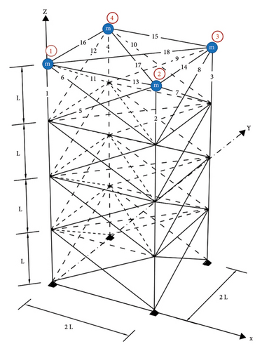
The symmetric nature of this structure adds to the complexity of the damage detection process. Two damage scenarios are considered according to Table 9. Like other examples, only first five modal values are used and noise effects are considered.

Table 9. Damage scenarios considered for the 72-bar spatial truss.

Scenario	I			II
Element number	1	21	37	8
Damage ratio (%)	25	20	30	25

Famine Algorithm and TLBO algorithm are used for the minimization task. For better comparison, the maximum number of function evaluations is set to 30000 and six three-membered groups of search parties or 18 search agents are allocated to the task.

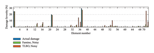
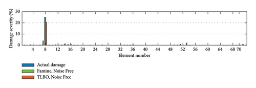
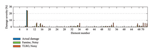
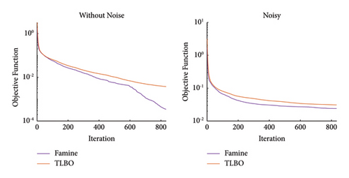
The overall performance of the suggested method can be seen in Figure 21, and the location and severity of the damage elements have been accurately detected by the Famine Algorithm. However, there are minor inaccuracies in the results of the Famine Algorithm but more major errors can be seen in TLBO results. This can be further seen in EI results presented in Table 10. The EI results show the maximum of 10.13 times more accuracy in noise-free conditions in case one for the Famine Algorithm. As expected, noise presentation added to the inaccuracy of the process. The reason for these results can further be interpreted from Figure 22 that shows the quicker convergence for Famine Algorithm, thus giving more accurate detection.

Table 10. Statistical EI results of the 72-bar spatial truss.

Scenario		I		II
Noise condition	Optimization algorithm	EI		EI
Noise condition	Optimization algorithm	Ave	Std	Ave	Std
Noise-free	Famine	3.20E − 02	2.62E − 02	4.07E − 02	6.48E − 02
Noise-free	TLBO	3.24E − 01	3.87E − 01	3.04E − 01	5.11E − 01

Noisy	Famine	7.73E − 01	4.73E − 01	7.16E − 01	4.09E − 01
Noisy	TLBO	1.86E + 0	1.23E + 0	1.31E + 0	8.95E − 01

4.3. Experimental Validation

An experimental example [52, 53] is considered in this section, to test the performance of the suggested method in real-life problems. Unlike the damage detection procedure in numerical examples, the experimental examples need two steps to locate the damage correctly. In the first step, the healthy FEM model is updated using the healthy experimental modal data so that the FEM model can be a good representative of the actual structure. In the second phase, the updated healthy FEM model is compared to the modal data from the damaged structure to locate the damage.

4.3.1. Three-Story Shear Frame

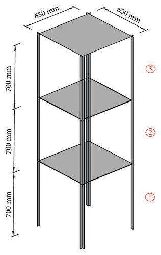
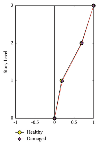
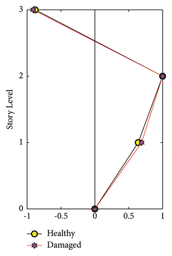
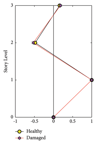
The shear frame structure illustrated in Figure 23 stands 2.1 m tall and has three stories. The floors are made from 650 × 650 × 30 mm stainless steel plates, and the columns are 30 × 30 mm equal angles made from aluminum. Furthermore, columns with 4.5 or 3.0 mm thicknesses are used to model the undamaged and damaged elements, respectively, and the columns are bolted to the floors and by aluminum brackets. The model is mounted on a shake table, and the data are collected by one uniaxial accelerometer on each floor and shake table in the direction of ground motion. The damage scenario is introduced by using the thin columns in the first story, which will result in a seven percent stiffness loss in the collective stiffness of the first story. Modal data are extracted for both healthy and damaged states using the data collected from the sensors and can be seen in Figure 24 and Table 11. A numerical lumped mass shear frame model with three degrees of freedom in the excitation direction is created for this structure. The Famine Algorithm and the base TLBO algorithm were utilized throughout the model updating and damage detection phases. The maximum number of NFEs allocated is 2000, and 12 search agents, or four groups of three search agents in case of Famine Algorithm, are assigned to:

Table 11. Experimental frequencies for three-story shear frame.

Mode	Healthy (Hz)	Damaged (Hz)
1^st	1.93	1.879
2^nd	5.52	5.43
3^rd	8.55	8.30

(1) Initial Model Updating Phase. Because there are no exact stiffness measurements in the healthy state of this structure, an initial rough estimation is needed to start the model updating process. For the second and third stories, stiffness values are estimated to be about 9,300 N/m, whereas for the first floor, because of the additional brackets that were used to abate any unwanted torsional movements, the stiffness is considered to be equal to 40,000 N/m.

Using the roughly calculated stiffnesses, the finite element model is created and is ready for the initial model updating phase using the healthy state data. The results of updated stiffnesses for both algorithms can be found in Table 12. The modal assurance criteria (MAC) and frequency change ratio (ΔFr) values are calculated for experimental and obtained mode shapes to evaluate the accuracy of these results and are presented in Table 13. Better agreement between experimental and obtained mode shapes and natural frequencies can be seen in the results of the Famine Algorithm compared to the TLBO algorithm.

Table 12. Story stiffnesses of three-story shear frame after initial model updating phase.

Story	Stiffness (N/m)
Story	Famine	TLBO
1^st	24133.86	24955.73
2^nd	9543.52	9430.65
3^rd	8135.45	8178.07

Table 13. Modal assurance criteria and frequency change ratio values of three-story shear frame in initial model updating phase.

Mode	MAC		ΔFr (%)
Mode	Famine	TLBO	Famine	TLBO
1^st	0.9993	0.9996	10.48	10.67
2^nd	1.0000	0.9997	0.00	0.57
3^rd	0.9991	0.9996	7.42	6.87

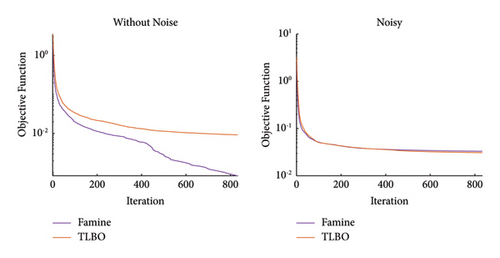
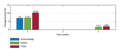
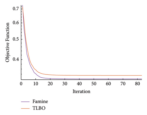
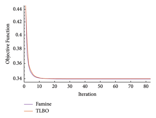
(2) Damage Detection Phase. By having the updated healthy model, damage detection can be carried out. The result of the damage detection process is presented in Figure 25. The Famine Algorithm seems to have more accurately detected the damage than the TLBO algorithm. Minor errors are seen in the third story due to noise effects and fem model simplifications. To better compare the performance of the two algorithms, convergence curves are plotted for both phases. Figure 26 shows that the Famine Algorithm converged more quickly, especially in the first phase, and found smaller minima than the base TLBO algorithm.

5. Conclusion

This study presented a new optimization-based model updating method for structural damage detection. Firstly, a multipopulation scheme named Famine Algorithm is introduced, which tries to lower the number of cost function evaluations needed for optimization algorithms to converge. This claim is tested and confirmed in 2D space for multiple examples. Secondly, a novel damage-sensitive feature named pseudo-kinetic energy is developed and is used in the objective function for the damage-detecting process. Three numerical examples and one experimental example are provided to illustrate the method’s capabilities. Firstly, a comparison between PKE and conventional KE features is presented for the 25-bar planar truss. The results for this truss show that the new feature can detect damage much more accurately than the conventional KE. Moreover, as illustrated in 2D space for the example of 2-bar truss, the PKE has a much simpler search space than KE. At its best performance, compared to MKE, PKE’s error values were 3.55 × 10⁹ times smaller.

In the second example, damage detection is carried out for 25-bar spatial truss using multiple well-known optimization algorithms to compare against the Famine Algorithm. The convergence histories show that in all scenarios, the Famine Algorithm was the quickest to converge and was able to reach smaller objective function values than its competitors placing TLBO, GWO, and PSO algorithms in lower ranks, respectively. To further clarify, by just adding the Famine Algorithm to the base TLBO algorithm, the error values were 1.14 × 10⁶ times smaller in its best-case scenario.

The last numerical example is allocated to evaluate the performance of the proposed method in frame structures. Performance improvements are noticeable when the Famine Algorithm is added to the base optimization algorithm and the location and severity of damages are found with acceptable precision. Again, the result for the Famine Algorithm was 32.9 times more accurate than the base TLBO algorithm in its best. In all numerical examples, the noise effects were investigated and only the first five mode shapes were used to include the incomplete data effects.

In the last example, an experimental three-story shear frame is considered to test the performance of the suggested method in real-life problems in which the suggested framework was able to detect damage with minor errors. The process included two phases, the initial model updating phase and damage detection. The final results show that adding the Famine Algorithm leads to more accurate damage detection.

Conflicts of Interest

The authors declare that they have no conflicts of interest.

Authors’ Contributions

S.M., A.K.G-T., and H.R. contributed to this study. S.M. carried out conceptualization, data collection and analyses, interpretation of the results, and preparing the first draft of the manuscript. A.K.G-T. and H.R. contributed to the conceptualization, design and conducting of the study, and critical revision of the manuscript.

Open Research

Data Availability

The data that support the findings of this study as well as the optimization framework referred herein are available from the corresponding author upon reasonable request.

References

1 Doebling S. W., Farrar C. R., Prime M. B., and Shevitz D. W., Damage identification and health monitoring of structural and mechanical systems from changes in their vibration characteristics: a literature review, 1996, Los Alamos National Laboratory Report, United State.
Google Scholar
2 Alkayem N. F., Cao M., Zhang Y., Bayat M., and Su Z., Structural damage detection using finite element model updating with evolutionary algorithms: a survey, Neural Computing and Applications. (2018) 30, no. 2, 389–411, https://doi.org/10.1007/s00521-017-3284-1, 2-s2.0-85034646702.
10.1007/s00521-017-3284-1
PubMed Web of Science® Google Scholar
3 Azimi M., Eslamlou A. D., and Pekcan G., Data-driven structural health monitoring and damage detection through deep learning: state-of-the-art review, Sensors. (2020) 20, no. 10, https://doi.org/10.3390/S20102778.
10.3390/s20102778
Google Scholar
4 Bhowmik B., Tripura T., Hazra B., and Pakrashi V., First-order eigen-perturbation techniques for real-time damage detection of vibrating systems: theory and applications, Applied Mechanics Reviews. (2019) 71, no. 6, https://doi.org/10.1115/1.4044287, 2-s2.0-85070708588.
10.1115/1.4044287
PubMed Web of Science® Google Scholar
5 Bhowmik B., Tripura T., Hazra B., and Pakrashi V., Real time structural modal identification using recursive canonical correlation analysis and application towards online structural damage detection, Journal of Sound and Vibration. (2020) 468, 115101, https://doi.org/10.1016/J.JSV.2019.115101.
10.1016/j.jsv.2019.115101
Web of Science® Google Scholar
6 Du Y., Zhou S., Jing X., Peng Y., Wu H., and Kwok N., Damage detection techniques for wind turbine blades: a review, Mechanical Systems and Signal Processing. (2020) 141, 106445, https://doi.org/10.1016/j.ymssp.2019.106445.
10.1016/j.ymssp.2019.106445
Web of Science® Google Scholar
7 Avci O., Abdeljaber O., Kiranyaz S., Hussein M., Gabbouj M., and Inman D. J., A review of vibration-based damage detection in civil structures: from traditional methods to Machine Learning and Deep Learning applications, Mechanical Systems and Signal Processing. (2021) 147, 107077, https://doi.org/10.1016/J.YMSSP.2020.107077.
10.1016/j.ymssp.2020.107077
Web of Science® Google Scholar
8 Kaveh A., Hosseini S. M., and Akbari H., Efficiency of Plasma generation optimization for structural damage identification of skeletal structures based on a hybrid cost function, Iranian Journal of Science and Technology, Transactions of Civil Engineering. (2020) 45, no. 4, 2069–2090, https://doi.org/10.1007/s40996-020-00504-8.
10.1007/s40996-020-00504-8
Web of Science® Google Scholar
9 Kaveh A., Akbari H., and Hosseini S. M., Plasma generation optimization: a new physically-based metaheuristic algorithm for solving constrained optimization problems, Engineering Computations. (2020) 38, no. 4, 1554–1606, https://doi.org/10.1108/EC-05-2020-0235.
10.1108/EC-05-2020-0235
Web of Science® Google Scholar
10 Ghannadi P. and Kourehli S. S., Multiverse optimizer for structural damage detection: numerical study and experimental validation, The Structural Design of Tall and Special Buildings. (2020) 29, no. 13, https://doi.org/10.1002/tal.1777.
10.1002/tal.1777
Web of Science® Google Scholar
11 Mirjalili S., Mirjalili S. M., and Hatamlou A., Multi-Verse Optimizer: a nature-inspired algorithm for global optimization, Neural Computing and Applications. (2016) 27, no. 2, 495–513, https://doi.org/10.1007/s00521-015-1870-7, 2-s2.0-84955627094.
10.1007/s00521-015-1870-7
Web of Science® Google Scholar
12 Ghahremani B., Bitaraf M., and Rahami H., A fast-convergent approach for damage assessment using CMA-ES optimization algorithm and modal parameters, Journal of Civil Structural Health Monitoring. (2020) 10, no. 3, 497–511, https://doi.org/10.1007/s13349-020-00397-1.
10.1007/s13349-020-00397-1
Web of Science® Google Scholar
13 Hansen N., Müller S. D., and Koumoutsakos P., Reducing the time complexity of the derandomized evolution strategy with covariance matrix adaptation (CMA-ES), Evolutionary Computation. (2003) 11, no. 1, 1–18, https://doi.org/10.1162/106365603321828970, 2-s2.0-0042879997.
10.1162/106365603321828970
PubMed Web of Science® Google Scholar
14 Zare Hosseinzadeh A., Bagheri A., Ghodrati Amiri G., and Koo K. Y., A flexibility-based method via the iterated improved reduction system and the cuckoo optimization algorithm for damage quantification with limited sensors, Smart Materials and Structures. (2014) 23, no. 4, 045019, https://doi.org/10.1088/0964-1726/23/4/045019, 2-s2.0-84896320849.
10.1088/0964-1726/23/4/045019
Web of Science® Google Scholar
15 Yang X. S. and Deb S., Cuckoo search via Lévy flights, Proceedings of the 2009 World Congress on Nature and Biologically Inspired Computing, NABIC 2009-Proceedings, December, 2009, Coimbatore, India, IEEE Publications, https://doi.org/10.1109/NABIC.2009.5393690, 2-s2.0-77949623076.
10.1109/NABIC.2009.5393690
Google Scholar
16 Dinh-Cong D., Vo-Duy T., Ho-Huu V., and Nguyen-Thoi T., Damage assessment in plate-like structures using a two-stage method based on modal strain energy change and Jaya algorithm, Inverse Problems in Science and Engineering. (2019) 27, no. 2, 166–189, https://doi.org/10.1080/17415977.2018.1454445, 2-s2.0-85044570935.
10.1080/17415977.2018.1454445
Web of Science® Google Scholar
17 Venkata Rao R., Jaya: a simple and new optimization algorithm for solving constrained and unconstrained optimization problems, International Journal of Industrial Engineering Computations. (2016) 7, 19–34, https://doi.org/10.5267/j.ijiec.2015.8.004, 2-s2.0-84940054935.
10.5267/j.ijiec.2015.8.004
Google Scholar
18 Kaveh A., Hosseini S. M., and Zaerreza A., Boundary strategy for optimization-based structural damage detection problem using metaheuristic algorithms, Periodica Polytechnica: Civil Engineering. (2020) 65, no. 1, 150–167, https://doi.org/10.3311/PPci.16924.
10.3311/PPci.16924
Web of Science® Google Scholar
19 Kaveh A. and Zaerreza A., Shuffled shepherd optimization method: a new Meta-heuristic algorithm, Engineering Computations. (2020) 37, no. 7, 2357–2389, https://doi.org/10.1108/ec-10-2019-0481.
10.1108/EC-10-2019-0481
Web of Science® Google Scholar
20 Gandomi A. H., Talatahari S., Yang X. S., and Deb S., Design optimization of truss structures using cuckoo search algorithm, The Structural Design of Tall and Special Buildings. (2013) 22, no. 17, 1330–1349, https://doi.org/10.1002/tal.1033, 2-s2.0-84886439592.
10.1002/tal.1033
Web of Science® Google Scholar
21 Kaveh A., Hosseini S. M., and Zaerreza A., Improved Shuffled Jaya algorithm for sizing optimization of skeletal structures with discrete variables, Structures. (2021) 29, 107–128, https://doi.org/10.1016/j.istruc.2020.11.008.
10.1016/j.istruc.2020.11.008
Web of Science® Google Scholar
22 Cantero-Chinchilla S., Papadimitriou C., Chiachío J., Chiachío M., Koumoutsakos P., Fabro A. T., and Chronopoulos D., Robust optimal sensor configuration using the value of information, Structural Control and Health Monitoring. (2022) 29, no. 12, https://doi.org/10.1002/STC.3143.
10.1002/stc.3143
PubMed Web of Science® Google Scholar
23 Kaveh A. and Bakhshpoori T., Metaheuristics: Outlines, MATLAB Codes and Examples, 2019, Springer Cham, New York, USA.
10.1007/978-3-030-04067-3
Google Scholar
24 Holland J. H., Genetic algorithms, Scientific American. (1992) 267, no. 1, 66–72, https://doi.org/10.1038/scientificamerican0792-66, 2-s2.0-0026988817.
10.1038/scientificamerican0792-66
PubMed Web of Science® Google Scholar
25 Gorges-Schleuter M., Comparison of local mating strategies in massively parallel genetic algorithms, Parallel problem solving from nature. (1992) 2.
Google Scholar
26 Xia X., Gui L., and Zhan Z. H., A multi-swarm particle swarm optimization algorithm based on dynamical topology and purposeful detecting, Applied Soft Computing. (2018) 67, 126–140, https://doi.org/10.1016/j.asoc.2018.02.042, 2-s2.0-85043502809.
10.1016/j.asoc.2018.02.042
Web of Science® Google Scholar
27 Blackwell T., Particle swarm optimization in dynamic environments, Studies in Computational Intelligence. (2007) 51, 29–49, https://doi.org/10.1007/978-3-540-49774-5_2, 2-s2.0-34147184847.
10.1007/978-3-540-49774-5_2
Google Scholar
28 Li C., Nguyen T. T., Yang M., Mavrovouniotis M., and Yang S., An adaptive multipopulation framework for locating and tracking multiple optima, IEEE Transactions on Evolutionary Computation. (2016) 20, no. 4, 590–605, https://doi.org/10.1109/TEVC.2015.2504383, 2-s2.0-84982799257.
10.1109/TEVC.2015.2504383
Web of Science® Google Scholar
29 Halder U., Das S., and Maity D., A cluster-based differential evolution algorithm with external archive for optimization in dynamic environments, IEEE Transactions on Cybernetics. (2013) 43, no. 3, 881–897, https://doi.org/10.1109/TSMCB.2012.2217491, 2-s2.0-84890441738.
10.1109/TSMCB.2012.2217491
PubMed Web of Science® Google Scholar
30 Hongru L., Jinxing H., and Shouyong J., A hybrid PSO based on dynamic clustering for global optimization, IFAC-PapersOnLine. (2018) 51, no. 18, 269–274, https://doi.org/10.1016/J.IFACOL.2018.09.311, 2-s2.0-85054449296.
10.1016/j.ifacol.2018.09.311
Google Scholar
31 Li C. and Yang S., A Clustering particle swarm optimizer for dynamic optimization, Proceedings of the 2009 IEEE Congress on Evolutionary Computation, CEC 2009, May 2009, Trondheim, Norway, 439–446, https://doi.org/10.1109/CEC.2009.4982979, 2-s2.0-70449890231.
10.1109/CEC.2009.4982979
Google Scholar
32 Ma H., Shen S., Yu M., Yang Z., Fei M., and Zhou H., Multi-population techniques in nature inspired optimization algorithms: a comprehensive survey, Swarm and Evolutionary Computation. (2019) 44, 365–387, https://doi.org/10.1016/J.SWEVO.2018.04.011, 2-s2.0-85046356963.
10.1016/j.swevo.2018.04.011
Web of Science® Google Scholar
33 Chaudhary R. and Banati H., Study of population partitioning techniques on efficiency of swarm algorithms, Swarm and Evolutionary Computation. (2020) 55, 100672, https://doi.org/10.1016/j.swevo.2020.100672.
10.1016/j.swevo.2020.100672
Web of Science® Google Scholar
34 Duan Q. Y., Gupta V. K., and Sorooshian S., Shuffled complex evolution approach for effective and efficient global minimization, Journal of Optimization Theory and Applications. (1993) 76, no. 3, 501–521, https://doi.org/10.1007/BF00939380, 2-s2.0-0027558431.
10.1007/BF00939380
Web of Science® Google Scholar
35 Eusuff M., Lansey K., and Pasha F., Shuffled frog-leaping algorithm: a memetic meta-heuristic for discrete optimization, Engineering Optimization. (2006) 38, no. 2, 129–154, https://doi.org/10.1080/03052150500384759, 2-s2.0-33244474874.
10.1080/03052150500384759
Web of Science® Google Scholar
36 Yammani C., Maheswarapu S., and Matam S. K., A Multi-objective Shuffled Bat algorithm for optimal placement and sizing of multi distributed generations with different load models, International Journal of Electrical Power and Energy Systems. (2016) 79, 120–131, https://doi.org/10.1016/J.IJEPES.2016.01.003, 2-s2.0-84954357506.
10.1016/j.ijepes.2016.01.003
Web of Science® Google Scholar
37 Banati H. and Chaudhary R., Enhanced shuffled bat algorithm (EShBAT), Proceedings of the 2016 International Conference on Advances in Computing, Communications and Informatics, ICACCI, September 2016, Jaipur, India, 731–738, https://doi.org/10.1109/ICACCI.2016.7732134, 2-s2.0-85007345803.
10.1109/ICACCI.2016.7732134
Google Scholar
38 Whitley D., The GENITOR algorithm and selection pressure: why rank-based allocation of reproductive trials is best, Proceedings of the Third International Conference on Genetic Algorithms. (1989) 1.
Google Scholar
39 Baker J. E., Reducing bias and inefficiency in the selection algorithm, Proceedings of the Second International Conference on Genetic Algorithms on Genetic Algorithms and Their Applications. (1987) Lawrence Erlbaum Associates Inc, Cambridge, MA, USA.
Google Scholar
40 Goldberg D. E., Genetic Algorithms in Search, Optimization, and Machine Learning, Addison-Wesley. (1989) Reading, MA, USA.
Google Scholar
41 Rao R. V., Savsani V. J., and Vakharia D. P., Teaching-learning-based optimization: a novel method for constrained mechanical design optimization problems, Computer-Aided Design. (2011) 43, no. 3, 303–315, https://doi.org/10.1016/j.cad.2010.12.015, 2-s2.0-78951475022.
10.1016/j.cad.2010.12.015
Web of Science® Google Scholar
42 Hadjian Shahri A. and Ghorbani-Tanha A. K., Damage detection via closed-form sensitivity matrix of modal kinetic energy change ratio, Journal of Sound and Vibration. (2017) 401, 268–281, https://doi.org/10.1016/j.jsv.2017.04.039, 2-s2.0-85019665578.
10.1016/j.jsv.2017.04.039
Web of Science® Google Scholar
43 Meng H. and Lin X., Damage orientation method based on the modal kinetic energy, Applied Mechanics and Materials. (2012) 256–259, no. PART 1, 1112–1116, https://doi.org/10.4028/WWW.SCIENTIFIC.NET/AMM.256-259.1112, 2-s2.0-84872937434.
10.4028/www.scientific.net/AMM.256-259.1112
Google Scholar
44 Montazer M. and Seyedpoor S. M., A new flexibility based damage index for damage detection of truss structures, Shock and Vibration. (2014) 2014, 1–12, https://doi.org/10.1155/2014/460692, 2-s2.0-84898031904.
10.1155/2014/460692
Web of Science® Google Scholar
45 Kaveh A., Hosseini Vaez S. R., Hosseini P., and Fathali M. A., A new two-phase method for damage detection in skeletal structures, Iranian Journal of Science and Technology, Transactions of Civil Engineering-Transactions of Civil Engineering. (2019) 43, no. S1, 49–65, https://doi.org/10.1007/s40996-018-0190-4, 2-s2.0-85065194933.
10.1007/s40996-018-0190-4
Web of Science® Google Scholar
46 Kaveh A. and Maniat M., Damage detection based on MCSS and PSO using modal data, Smart Structures and Systems. (2015) 15, no. 5, 1253–1270, https://doi.org/10.12989/sss.2015.15.5.1253, 2-s2.0-84929612181.
10.12989/sss.2015.15.5.1253
Web of Science® Google Scholar
47 Villalba J. D. and Laier J. E., Localising and quantifying damage by means of a multi-chromosome genetic algorithm, Advances in Engineering Software. (2012) 50, no. 1, 150–157, https://doi.org/10.1016/J.ADVENGSOFT.2012.02.002, 2-s2.0-84861918087.
10.1016/j.advengsoft.2012.02.002
Web of Science® Google Scholar
48 Perera R. and Torres R., Structural damage detection via modal data with genetic algorithms, Journal of Structural Engineering. (2006) 132, no. 9, 1491–1501, https://doi.org/10.1061/(ASCE)0733-9445(2006)132:9(1491), 2-s2.0-33747346960.
10.1061/(ASCE)0733-9445(2006)132:9(1491)
Web of Science® Google Scholar
49 Seyedpoor S. M., A two stage method for structural damage detection using a modal strain energy based index and particle swarm optimization, International Journal of Non-linear Mechanics. (2012) 47, no. 1, 1–8, https://doi.org/10.1016/j.ijnonlinmec.2011.07.011, 2-s2.0-80054954470.
10.1016/j.ijnonlinmec.2011.07.011
Web of Science® Google Scholar
50 Messina A., Williams E. J., and Contursi T., Structural damage detection by a sensitivity and statistical-based method, Journal of Sound and Vibration. (1998) 216, no. 5, 791–808, https://doi.org/10.1006/JSVI.1998.1728, 2-s2.0-0032497444.
10.1006/jsvi.1998.1728
Web of Science® Google Scholar
51 Mirjalili S., Mirjalili S. M., and Lewis A., Grey Wolf optimizer, Advances in Engineering Software. (2014) 69, 46–61, https://doi.org/10.1016/j.advengsoft.2013.12.007, 2-s2.0-84893010002.
10.1016/j.advengsoft.2013.12.007
Web of Science® Google Scholar
52 De Lautour O. R. and Omenzetter P., Nearest neighbor and learning vector quantization classification for damage detection using time series analysis, Structural Control and Health Monitoring. (2009) 17, no. 6, 614–631, https://doi.org/10.1002/stc.335, 2-s2.0-84856361730.
10.1002/stc.335
Web of Science® Google Scholar
53 de Lautour O. R. and Omenzetter P., Damage classification and estimation in experimental structures using time series analysis and pattern recognition, Mechanical Systems and Signal Processing. (2010) 24, no. 5, 1556–1569, https://doi.org/10.1016/j.ymssp.2009.12.008, 2-s2.0-77953325047.
10.1016/j.ymssp.2009.12.008
Web of Science® Google Scholar

All articles

Famine Algorithm and Pseudo-Kinetic Energy for Structural Damage Detection

Abstract

1. Introduction

2. Famine Algorithm

2.1. Search Agent Grouping

2.2. Resource Allocation

2.2.1. Rank-Based Fitness Assignment

2.2.2. Roulette Wheel Selection

2.3. Search Strategy

2.3.1. Teaching-Learning-Based Optimization Algorithm

2.4. Steps of the Famine Algorithm

3. Damage Detection Methodology

3.1. Damage Formulation

3.2. Noise Effect

3.3. Objective Function

3.3.1. Modal Kinetic Energy

3.3.2. Pseudo-Kinetic Energy

3.3.3. Proposed Objective Function

3.3.4. Error Calculation

3.4. Illustrated Comparison of the Objective Functions

4. Method Efficiency Evaluation

4.1. Performance Monitoring and Convergence Behavior

4.2. Numerical Examples

4.2.1. 25-Bar Planar Truss

4.2.2. 25-Bar Spatial Truss

4.2.3. 23-Element Asymmetrical Planar Frame

4.2.4. 72-Bar Spatial Truss

4.3. Experimental Validation

4.3.1. Three-Story Shear Frame

5. Conclusion

Conflicts of Interest

Authors’ Contributions

Open Research

Data Availability

References

Figures

References

Related

Information