Efficient Numerical Method for Solving a Quadratic Riccati Differential Equation
Abstract
This study presents families of the fourth-order Runge–Kutta methods for solving a quadratic Riccati differential equation. From these families, the England version is more efficient than other fourth-order Runge–Kutta methods and practically well-suited for solving initial value problems in general and quadratic Riccati differential equation in particular. The stability analysis of the present method is well-established. In order to verify the accuracy, we compared the numerical solutions obtained using the England version of fourth-order Runge–Kutta method with the recently published works reported in the literature. Several counter examples are solved using the present methods to demonstrate their reliability and efficiency.
1. Introduction
Differential equations are a popular approach to solve problems in science and engineering. The differential equation used to approximate a large number of real-world problems is difficult to solve analytically due to its complexity and nonlinearity. The challenges of finding analytical solutions to real-world problems led to the development of numerical methods.
Nonlinear ordinary differential equations are essential in many areas of both applied and pure mathematics, including engineering, applied mechanics, quantum physics, analytical chemistry, astronomy, and biology. Researchers have been interested in the analytical and numerical solutions to nonlinear ordinary differential equations. Riccati differential equation is a type of nonlinear differential equation that is particularly important in many practical scientific disciplines. For example, Riccati differential equation is closely connected to a 1D static Schrödinger equation [1]. Riccati differential equation is named after the Italian nobleman Count Jacopo Francesco Riccati [2]. These equations have applications not only in random processes, optimal control, and diffusion problems [3] but also in engineering and applied science, such as damping laws, rheology, diffusion processes, transmission line phenomena, network synthesis, financial mathematics, and stochastic realization theory problems [4].
Many authors have proposed various numerical methods to solve Equations (1) and (2). For instance, piecewise variational iteration method in Ghorbani and Momani’s [5] study, differential transform method in Biazar and Eslami’s [4] study, cubic B-spline scaling functions and Chebyshev cardinal functions in Lakestani and Dehghan’s [6] study, application of optimal homotopy asymptotic method in Mabood et al.’s [7] study, combination of Laplace transform and new homotopy perturbation methods in Vahidi et al.’s [8] study, Legendre scaling functions in Baghchehjoughi et al.’s [9] study, Lie group method and Runge–Kutta fourth-order method in Altoum’s [10] study, fourth-order Runge–Kutta method in File and Aga’s [11] study, the Bezier curves method in Ghomanjani and Khorram’s [12] study, a weighted type of Adams–Bashforth rules in Masjed-Jamei and Shayegan’s [13] study, and the fifth order predictor corrector method in Kiltu et al.’s [14] study. The classical fourth-order Runge–Kutta method is widely used for solving quadratic Riccati differential equations. However, the accuracy is very less. Therefore, in this study, families of fourth-order Runge–Kutta methods are devised for solving quadratic Riccati differential equations. From the tables of values, one can observe that England’s version of the fourth-order Runge–Kutta method gives a more accurate numerical solution than the other Runge–Kutta methods as well as recently published works. From in this study, we therefore conclude that the England version of fourth-order Runge–Kutta method is more accurate and effective to solve a quadratic Riccati differential equation.
2. Description of the Method
From the above families of fourth-order Runge–Kutta methods, we consider the England version of the fourth-order Runge–Kutta method given in Equation (8) to show the stability analysis.
3. Stability Analysis
4. Counter Examples
Example 1. Consider the variable coefficient RDE [11]:
Example 2. Consider the constant coefficient RDE [11]:
Example 3. Consider the variable coefficient RDE [11]:
Example 4. Consider the variable coefficient RDE:
Example 5. Consider the variable coefficient RDE:
5. Numerical Results and Discussions
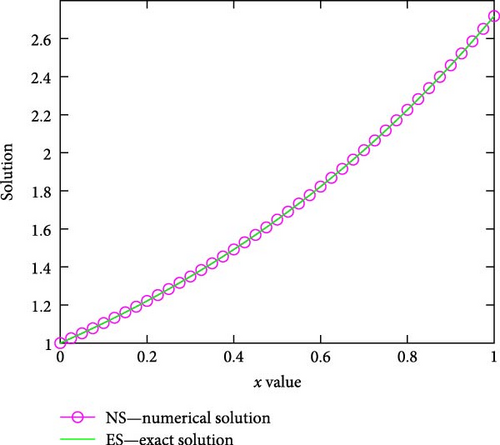
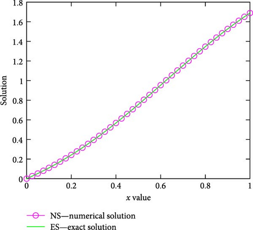
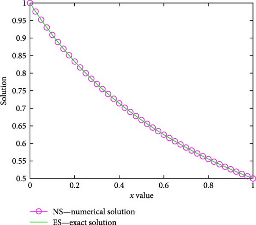
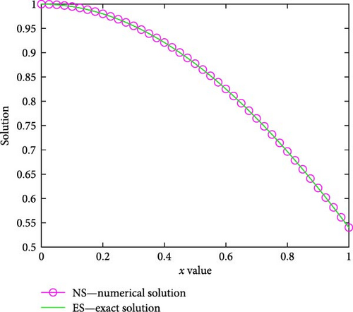
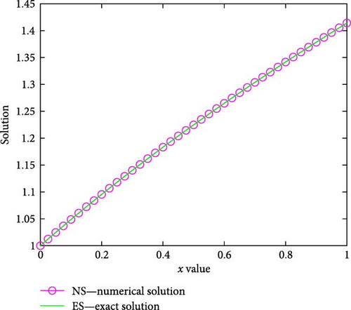
From Tables 1), (2) and (3, one can observe that England version of fourth-order Runge–Kutta method gives more accurate solution than the other versions of fourth-order Runge–Kutta methods for Examples (1) (2) and (3), respectively. For Examples (1) and (2), the numerical results using England version of fourth-order Runge–Kutta method are more accurate than those of the cubic B-spline method in Ala’yed et al.’s [17] study, the classical fourth-order Runge–Kutta method in File and Aga’s [11] study, and the BCM in Ghomanjani and Khorram’s [12] study for N = 10, as depicted in Tables 4 and 5, respectively. This implies that for the chosen N = 10, the AEs of the present method using the England version of the Runge–Kutta method are less than 10−8. The numerical results using England version of fourth-order Runge–Kutta method for Examples (4) and (5) are more accurate than in Masjed-Jamei and Shayegan’s [13] study for N = 100, as displayed in Tables 6 and 7, respectively. Table 8 demonstrates the numerical rate of convergence. In all the tables, we can observe that the AEs decrease as the number of mesh points increases. The graphs of numerical and exact solutions are sketched in Figures (1, 2)–(3) for Examples (1)–(5) for N = 40.
| x↓ | N = 10 | N = 20 | N = 40 | N = 80 | N = 160 | N = 320 | N = 640 |
|---|---|---|---|---|---|---|---|
| Case I: classical RK4 method | |||||||
| 0.1 | 1.1153e-07 | 7.1708e-09 | 4.5427e-10 | 2.8580e-11 | 1.7923e-12 | 1.1258e-13 | 7.3275e-15 |
| 0.2 | 2.6297e-07 | 1.6906e-08 | 1.0710e-09 | 6.7377e-11 | 4.2253e-12 | 2.6446e-13 | 1.7097e-14 |
| 0.3 | 4.6838e-07 | 3.0109e-08 | 1.9073e-09 | 1.1999e-10 | 7.5240e-12 | 4.7051e-13 | 3.0642e-14 |
| 0.4 | 7.4674e-07 | 4.8000e-08 | 3.0404e-09 | 1.9127e-10 | 1.1994e-11 | 7.4984e-13 | 4.9738e-14 |
| 0.5 | 1.1237e-06 | 7.2225e-08 | 4.5748e-09 | 2.8779e-10 | 1.8045e-11 | 1.1273e-12 | 7.5051e-14 |
| 0.6 | 1.6338e-06 | 1.0501e-07 | 6.6511e-09 | 4.1841e-10 | 2.6235e-11 | 1.6427e-12 | 1.1013e-13 |
| 0.7 | 2.3239e-06 | 1.4935e-07 | 9.4596e-09 | 5.9507e-10 | 3.7311e-11 | 2.3390e-12 | 1.5632e-13 |
| 0.8 | 3.2569e-06 | 2.0931e-07 | 1.3257e-08 | 8.3395e-10 | 5.2287e-11 | 3.2805e-12 | 2.1760e-13 |
| 0.9 | 4.5182e-06 | 2.9036e-07 | 1.8390e-08 | 1.1568e-09 | 7.2531e-11 | 4.5524e-12 | 2.9932e-13 |
| 1 | 6.2225e-06 | 3.9989e-07 | 2.5327e-08 | 1.5932e-09 | 9.9895e-11 | 6.2537e-12 | 3.8369e-13 |
| Case II: England version of RK4 method | |||||||
| 0.1 | 3.6077e-09 | 2.2755e-10 | 1.4254e-11 | 8.9129e-13 | 5.5733e-14 | 2.8866e-15 | 1.3323e-15 |
| 0.2 | 7.5843e-09 | 4.7887e-10 | 3.0005e-11 | 1.8767e-12 | 1.1746e-13 | 7.7716e-15 | 2.4425e-15 |
| 0.3 | 1.1965e-08 | 7.5640e-10 | 4.7408e-11 | 2.9652e-12 | 1.8630e-13 | 1.3101e-14 | 1.9984e-15 |
| 0.4 | 1.6788e-08 | 1.0628e-09 | 6.6638e-11 | 4.1682e-12 | 2.6201e-13 | 1.8208e-14 | 2.2204e-16 |
| 0.5 | 2.2093e-08 | 1.4011e-09 | 8.7883e-11 | 5.4976e-12 | 3.4595e-13 | 2.3981e-14 | 1.5543e-15 |
| 0.6 | 2.7922e-08 | 1.7744e-09 | 1.1135e-10 | 6.9678e-12 | 4.3876e-13 | 2.7534e-14 | 4.4409e-15 |
| 0.7 | 3.4318e-08 | 2.1862e-09 | 1.3728e-10 | 8.5918e-12 | 5.4046e-13 | 3.1086e-14 | 7.1054e-15 |
| 0.8 | 4.1327e-08 | 2.6404e-09 | 1.6592e-10 | 1.0387e-11 | 6.5414e-13 | 3.6415e-14 | 1.0214e-14 |
| 0.9 | 4.8992e-08 | 3.1410e-09 | 1.9756e-10 | 1.2370e-11 | 7.7893e-13 | 4.1744e-14 | 1.4655e-14 |
| 1 | 5.7356e-08 | 3.6925e-09 | 2.3249e-10 | 1.4556e-11 | 9.0861e-13 | 6.2617e-14 | 8.4377e-15 |
| Case III: a new formula of RK4 method | |||||||
| 0.1 | 3.4181e-07 | 2.1968e-08 | 1.3913e-09 | 8.7523e-11 | 5.4883e-12 | 3.4306e-13 | 2.1316e-14 |
| 0.2 | 8.0409e-07 | 5.1676e-08 | 3.2729e-09 | 2.0588e-10 | 1.2910e-11 | 8.0780e-13 | 4.9294e-14 |
| 0.3 | 1.4291e-06 | 9.1841e-08 | 5.8166e-09 | 3.6590e-10 | 2.2943e-11 | 1.4355e-12 | 8.9262e-14 |
| 0.4 | 2.2738e-06 | 1.4612e-07 | 9.2546e-09 | 5.8216e-10 | 3.6501e-11 | 2.2840e-12 | 1.4455e-13 |
| 0.5 | 3.4152e-06 | 2.1948e-07 | 1.3900e-08 | 8.7438e-10 | 5.4823e-11 | 3.4304e-12 | 2.1871e-13 |
| 0.6 | 4.9573e-06 | 3.1857e-07 | 2.0176e-08 | 1.2692e-09 | 7.9574e-11 | 4.9818e-12 | 3.1841e-13 |
| 0.7 | 7.0403e-06 | 4.5243e-07 | 2.8653e-08 | 1.8024e-09 | 1.1301e-10 | 7.0774e-12 | 4.5297e-13 |
| 0.8 | 9.8535e-06 | 6.3322e-07 | 4.0103e-08 | 2.5226e-09 | 1.5816e-10 | 9.9059e-12 | 6.3283e-13 |
| 0.9 | 1.3653e-05 | 8.7737e-07 | 5.5565e-08 | 3.4952e-09 | 2.1914e-10 | 1.3727e-11 | 8.7397e-13 |
| 1 | 1.8782e-05 | 1.2071e-06 | 7.6445e-08 | 4.8086e-09 | 3.0150e-10 | 1.8870e-11 | 1.1742e-12 |
| Case IV: a second new formula of RK4 method | |||||||
| 0.1 | 3.4772e-08 | 2.2386e-09 | 1.4192e-10 | 8.9324e-12 | 5.6022e-13 | 3.4861e-14 | 1.3323e-15 |
| 0.2 | 8.2602e-08 | 5.3161e-09 | 3.3699e-10 | 2.1208e-11 | 1.3303e-12 | 8.3045e-14 | 3.5527e-15 |
| 0.3 | 1.4815e-07 | 9.5322e-09 | 6.0415e-10 | 3.8020e-11 | 2.3841e-12 | 1.4855e-13 | 8.6597e-15 |
| 0.4 | 2.3772e-07 | 1.5291e-08 | 9.6905e-10 | 6.0980e-11 | 3.8232e-12 | 2.3848e-13 | 1.5321e-14 |
| 0.5 | 3.5983e-07 | 2.3141e-08 | 1.4663e-09 | 9.2267e-11 | 5.7845e-12 | 3.6016e-13 | 2.5757e-14 |
| 0.6 | 5.2599e-07 | 3.3820e-08 | 2.1428e-09 | 1.3482e-10 | 8.4523e-12 | 5.2913e-13 | 3.8414e-14 |
| 0.7 | 7.5175e-07 | 4.8327e-08 | 3.0617e-09 | 1.9263e-10 | 1.2077e-11 | 7.5939e-13 | 5.6399e-14 |
| 0.8 | 1.0581e-06 | 6.8011e-08 | 4.3084e-09 | 2.7106e-10 | 1.6994e-11 | 1.0703e-12 | 7.8604e-14 |
| 0.9 | 1.4734e-06 | 9.4694e-08 | 5.9983e-09 | 3.7736e-10 | 2.3660e-11 | 1.4921e-12 | 1.0791e-13 |
| 1 | 2.0359e-06 | 1.3084e-07 | 8.2872e-09 | 5.2135e-10 | 3.2694e-11 | 2.0446e-12 | 1.2035e-13 |
| Case V: a third new formula of RK4 method | |||||||
| 0.1 | 2.6635e-08 | 1.7072e-09 | 1.0796e-10 | 6.7855e-12 | 4.2544e-13 | 2.7089e-14 | 2.6645e-15 |
| 0.2 | 6.1696e-08 | 3.9559e-09 | 2.5020e-10 | 1.5727e-11 | 9.8588e-13 | 6.2617e-14 | 5.5511e-15 |
| 0.3 | 1.0803e-07 | 6.9295e-09 | 4.3835e-10 | 2.7556e-11 | 1.7273e-12 | 1.0969e-13 | 7.7716e-15 |
| 0.4 | 1.6949e-07 | 1.0875e-08 | 6.8805e-10 | 4.3256e-11 | 2.7112e-12 | 1.7164e-13 | 9.1038e-15 |
| 0.5 | 2.5125e-07 | 1.6126e-08 | 1.0204e-09 | 6.4155e-11 | 4.0221e-12 | 2.5424e-13 | 1.2434e-14 |
| 0.6 | 3.6027e-07 | 2.3131e-08 | 1.4638e-09 | 9.2041e-11 | 5.7707e-12 | 3.6171e-13 | 1.7097e-14 |
| 0.7 | 5.0596e-07 | 3.2494e-08 | 2.0567e-09 | 1.2932e-10 | 8.1086e-12 | 5.0493e-13 | 2.3981e-14 |
| 0.8 | 7.0098e-07 | 4.5031e-08 | 2.8505e-09 | 1.7925e-10 | 1.1239e-11 | 6.9855e-13 | 3.4639e-14 |
| 0.9 | 9.6242e-07 | 6.1842e-08 | 3.9151e-09 | 2.4621e-10 | 1.5439e-11 | 9.5746e-13 | 4.9294e-14 |
| 1 | 1.3133e-06 | 8.4410e-08 | 5.3443e-09 | 3.3610e-10 | 2.1069e-11 | 1.3225e-12 | 9.4591e-14 |
| x↓ | N = 10 | N = 20 | N = 40 | N = 80 | N = 160 | N = 320 | N = 640 |
|---|---|---|---|---|---|---|---|
| Case I: classical RK4 method | |||||||
| 0.1 | 2.2551e-06 | 1.5184e-07 | 9.8491e-09 | 6.2708e-10 | 3.9557e-11 | 2.4840e-12 | 1.5543e-13 |
| 0.2 | 4.7763e-06 | 3.1936e-07 | 2.0641e-08 | 1.3119e-09 | 8.2681e-11 | 5.1891e-12 | 3.2457e-13 |
| 0.3 | 7.3083e-06 | 4.8505e-07 | 3.1235e-08 | 1.9814e-09 | 1.2476e-10 | 7.8259e-12 | 4.9027e-13 |
| 0.4 | 9.5635e-06 | 6.3023e-07 | 4.0441e-08 | 2.5610e-09 | 1.6111e-10 | 1.0101e-11 | 6.3527e-13 |
| 0.5 | 1.1301e-05 | 7.4039e-07 | 4.7374e-08 | 2.9957e-09 | 1.8833e-10 | 1.1803e-11 | 7.4463e-13 |
| 0.6 | 1.2408e-05 | 8.0984e-07 | 5.1724e-08 | 3.2678e-09 | 2.0534e-10 | 1.2869e-11 | 8.1413e-13 |
| 0.7 | 1.2940e-05 | 8.4328e-07 | 5.3815e-08 | 3.3985e-09 | 2.1351e-10 | 1.3382e-11 | 8.4910e-13 |
| 0.8 | 1.3100e-05 | 8.5316e-07 | 5.4419e-08 | 3.4357e-09 | 2.1581e-10 | 1.3529e-11 | 8.6020e-13 |
| 0.9 | 1.3141e-05 | 8.5375e-07 | 5.4381e-08 | 3.4308e-09 | 2.1543e-10 | 1.3503e-11 | 8.5909e-13 |
| 1 | 1.3245e-05 | 8.5473e-07 | 5.4260e-08 | 3.4174e-09 | 2.1441e-10 | 1.3427e-11 | 8.3977e-13 |
| Case II: England version of RK4 method | |||||||
| 0.1 | 1.8238e-06 | 1.2286e-07 | 7.9738e-09 | 5.0789e-10 | 3.2046e-11 | 2.0125e-12 | 1.2590e-13 |
| 0.2 | 3.7840e-06 | 2.5339e-07 | 1.6397e-08 | 1.0428e-09 | 6.5747e-11 | 4.1272e-12 | 2.5807e-13 |
| 0.3 | 5.7022e-06 | 3.7952e-07 | 2.4483e-08 | 1.5547e-09 | 9.7944e-11 | 6.1453e-12 | 3.8519e-13 |
| 0.4 | 7.4121e-06 | 4.9044e-07 | 3.1547e-08 | 2.0004e-09 | 1.2593e-10 | 7.8977e-12 | 4.9760e-13 |
| 0.5 | 8.7887e-06 | 5.7860e-07 | 3.7126e-08 | 2.3512e-09 | 1.4792e-10 | 9.2731e-12 | 5.8653e-13 |
| 0.6 | 9.7606e-06 | 6.4011e-07 | 4.0995e-08 | 2.5937e-09 | 1.6310e-10 | 1.0225e-11 | 6.4893e-13 |
| 0.7 | 1.0321e-05 | 6.7501e-07 | 4.3170e-08 | 2.7294e-09 | 1.7158e-10 | 1.0757e-11 | 6.8523e-13 |
| 0.8 | 1.0545e-05 | 6.8794e-07 | 4.3938e-08 | 2.7761e-09 | 1.7445e-10 | 1.0938e-11 | 6.9811e-13 |
| 0.9 | 1.0585e-05 | 6.8771e-07 | 4.3828e-08 | 2.7662e-09 | 1.7373e-10 | 1.0892e-11 | 6.9567e-13 |
| 1 | 1.0608e-05 | 6.8394e-07 | 4.3423e-08 | 2.7354e-09 | 1.7164e-10 | 1.0749e-11 | 6.7191e-13 |
| Case III: a new formula of RK4 method | |||||||
| 0.1 | 3.1177e-06 | 2.0981e-07 | 1.3600e-08 | 8.6546e-10 | 5.4580e-11 | 3.4268e-12 | 2.1448e-13 |
| 0.2 | 6.7609e-06 | 4.5128e-07 | 2.9131e-08 | 1.8500e-09 | 1.1655e-10 | 7.3131e-12 | 4.5755e-13 |
| 0.3 | 1.0520e-05 | 6.9611e-07 | 4.4738e-08 | 2.8350e-09 | 1.7840e-10 | 1.1188e-11 | 7.0077e-13 |
| 0.4 | 1.3866e-05 | 9.0980e-07 | 5.8229e-08 | 3.6821e-09 | 2.3147e-10 | 1.4508e-11 | 9.1094e-13 |
| 0.5 | 1.6326e-05 | 1.0640e-06 | 6.7872e-08 | 4.2849e-09 | 2.6914e-10 | 1.6861e-11 | 1.0610e-12 |
| 0.6 | 1.7701e-05 | 1.1493e-06 | 7.3182e-08 | 4.6159e-09 | 2.8981e-10 | 1.8155e-11 | 1.1446e-12 |
| 0.7 | 1.8177e-05 | 1.1798e-06 | 7.5107e-08 | 4.7367e-09 | 2.9737e-10 | 1.8630e-11 | 1.1773e-12 |
| 0.8 | 1.8211e-05 | 1.1836e-06 | 7.5383e-08 | 4.7551e-09 | 2.9854e-10 | 1.8707e-11 | 1.1846e-12 |
| 0.9 | 1.8255e-05 | 1.1858e-06 | 7.5485e-08 | 4.7600e-09 | 2.9881e-10 | 1.8723e-11 | 1.1871e-12 |
| 1 | 1.8519e-05 | 1.1963e-06 | 7.5933e-08 | 4.7814e-09 | 2.9994e-10 | 1.8780e-11 | 1.1759e-12 |
| Case IV: a second new formula of RK4 method | |||||||
| 0.1 | 1.9675e-06 | 1.3252e-07 | 8.5989e-09 | 5.4762e-10 | 3.4549e-11 | 2.1696e-12 | 1.3577e-13 |
| 0.2 | 4.1148e-06 | 2.7538e-07 | 1.7812e-08 | 1.1325e-09 | 7.1392e-11 | 4.4811e-12 | 2.8008e-13 |
| 0.3 | 6.2376e-06 | 4.1469e-07 | 2.6734e-08 | 1.6969e-09 | 1.0688e-10 | 6.7053e-12 | 4.2016e-13 |
| 0.4 | 8.1292e-06 | 5.3704e-07 | 3.4512e-08 | 2.1872e-09 | 1.3766e-10 | 8.6320e-12 | 5.4312e-13 |
| 0.5 | 9.6262e-06 | 6.3253e-07 | 4.0542e-08 | 2.5660e-09 | 1.6139e-10 | 1.0116e-11 | 6.3882e-13 |
| 0.6 | 1.0643e-05 | 6.9669e-07 | 4.4571e-08 | 2.8184e-09 | 1.7718e-10 | 1.1107e-11 | 7.0366e-13 |
| 0.7 | 1.1194e-05 | 7.3110e-07 | 4.6718e-08 | 2.9525e-09 | 1.8555e-10 | 1.1633e-11 | 7.3919e-13 |
| 0.8 | 1.1397e-05 | 7.4302e-07 | 4.7432e-08 | 2.9960e-09 | 1.8824e-10 | 1.1801e-11 | 7.5162e-13 |
| 0.9 | 1.1437e-05 | 7.4305e-07 | 4.7346e-08 | 2.9877e-09 | 1.8763e-10 | 1.1762e-11 | 7.4984e-13 |
| 1 | 1.1487e-05 | 7.4087e-07 | 4.7035e-08 | 2.9628e-09 | 1.8590e-10 | 1.1640e-11 | 7.2764e-13 |
| Case V: a third new formula of RK4 method | |||||||
| 0.1 | 1.7375e-06 | 1.1706e-07 | 7.5988e-09 | 4.8405e-10 | 3.0543e-11 | 1.9182e-12 | 1.1996e-13 |
| 0.2 | 3.5855e-06 | 2.4020e-07 | 1.5548e-08 | 9.8900e-10 | 6.2360e-11 | 3.9146e-12 | 2.4469e-13 |
| 0.3 | 5.3810e-06 | 3.5841e-07 | 2.3133e-08 | 1.4693e-09 | 9.2579e-11 | 5.8089e-12 | 3.6421e-13 |
| 0.4 | 6.9818e-06 | 4.6248e-07 | 2.9769e-08 | 1.8882e-09 | 1.1889e-10 | 7.4570e-12 | 4.7018e-13 |
| 0.5 | 8.2862e-06 | 5.4624e-07 | 3.5076e-08 | 2.2222e-09 | 1.3984e-10 | 8.7679e-12 | 5.5511e-13 |
| 0.6 | 9.2312e-06 | 6.0616e-07 | 3.8849e-08 | 2.4589e-09 | 1.5466e-10 | 9.6974e-12 | 6.1595e-13 |
| 0.7 | 9.7971e-06 | 6.4135e-07 | 4.1041e-08 | 2.5956e-09 | 1.6319e-10 | 1.0233e-11 | 6.5215e-13 |
| 0.8 | 8.2862e-06 | 6.5490e-07 | 4.1841e-08 | 2.6442e-09 | 1.6618e-10 | 1.0421e-11 | 6.6547e-13 |
| 0.9 | 9.2312e-06 | 6.5450e-07 | 4.1718e-08 | 2.6333e-09 | 1.6539e-10 | 1.0371e-11 | 6.6280e-13 |
| 1 | 1.0081e-05 | 6.4978e-07 | 4.1255e-08 | 2.5990e-09 | 1.6309e-10 | 1.0214e-11 | 6.3838e-13 |
| x↓ | N = 10 | N = 20 | N = 40 | N = 80 | N = 160 | N = 320 | N = 640 |
|---|---|---|---|---|---|---|---|
| Case I: classical RK4 method | |||||||
| 0.1 | 3.8296e-07 | 2.1510e-08 | 1.2712e-09 | 7.7213e-11 | 4.7566e-12 | 2.9510e-13 | 1.8319e-14 |
| 0.2 | 5.7951e-07 | 3.2725e-08 | 1.9396e-09 | 1.1798e-10 | 7.2735e-12 | 4.5164e-13 | 2.7978e-14 |
| 0.3 | 6.8133e-07 | 3.8623e-08 | 2.2939e-09 | 1.3968e-10 | 8.6161e-12 | 5.3524e-13 | 3.2752e-14 |
| 0.4 | 7.3394e-07 | 4.1722e-08 | 2.4816e-09 | 1.5123e-10 | 9.3322e-12 | 5.7987e-13 | 3.4639e-14 |
| 0.5 | 7.6091e-07 | 4.3344e-08 | 2.5808e-09 | 1.5737e-10 | 9.7137e-12 | 6.0407e-13 | 3.5416e-14 |
| 0.6 | 7.7483e-07 | 4.4202e-08 | 2.6340e-09 | 1.6067e-10 | 9.9198e-12 | 6.1640e-13 | 3.5860e-14 |
| 0.7 | 7.8257e-07 | 4.4692e-08 | 2.6648e-09 | 1.6260e-10 | 1.0040e-11 | 6.2339e-13 | 3.5638e-14 |
| 0.8 | 7.8799e-07 | 4.5037e-08 | 2.6865e-09 | 1.6396e-10 | 1.0126e-11 | 6.2883e-13 | 3.5638e-14 |
| 0.9 | 7.9326e-07 | 4.5365e-08 | 2.7069e-09 | 1.6523e-10 | 1.0205e-11 | 6.3338e-13 | 3.5194e-14 |
| 1 | 7.9961e-07 | 4.5748e-08 | 2.7304e-09 | 1.6669e-10 | 1.0295e-11 | 6.4021e-13 | 3.7692e-14 |
| Case II: England version of RK4 method | |||||||
| 0.1 | 2.1401e-08 | 8.5002e-10 | 3.8238e-11 | 1.9329e-12 | 1.0647e-13 | 6.2172e-15 | 4.4409e-16 |
| 0.2 | 3.7105e-08 | 1.6162e-09 | 7.9370e-11 | 4.2936e-12 | 2.4736e-13 | 1.4988e-14 | 1.1102e-15 |
| 0.3 | 4.6667e-08 | 2.1219e-09 | 1.0802e-10 | 5.9908e-12 | 3.5072e-13 | 2.1538e-14 | 1.1102e-15 |
| 0.4 | 5.1839e-08 | 2.4094e-09 | 1.2480e-10 | 7.0011e-12 | 4.1289e-13 | 2.5757e-14 | 7.7716e-16 |
| 0.5 | 5.4295e-08 | 2.5521e-09 | 1.3332e-10 | 7.5204e-12 | 4.4509e-13 | 2.7978e-14 | 2.2204e-16 |
| 0.6 | 5.5228e-08 | 2.6096e-09 | 1.3685e-10 | 7.7387e-12 | 4.5852e-13 | 2.8200e-14 | 1.1102e-16 |
| 0.7 | 5.5412e-08 | 2.6231e-09 | 1.3773e-10 | 7.7948e-12 | 4.6207e-13 | 2.8089e-14 | 6.6613e-16 |
| 0.8 | 5.5315e-08 | 2.6185e-09 | 1.3748e-10 | 7.7798e-12 | 4.6108e-13 | 2.7534e-14 | 1.1102e-15 |
| 0.9 | 5.5215e-08 | 2.6116e-09 | 1.3702e-10 | 7.7501e-12 | 4.5897e-13 | 2.7200e-14 | 1.8874e-15 |
| 1 | 5.5268e-08 | 2.6114e-09 | 1.3689e-10 | 7.7386e-12 | 4.5747e-13 | 2.8089e-14 | 2.7756e-16 |
| Case III: a new formula of RK4 method | |||||||
| 0.1 | 1.1061e-06 | 6.2829e-08 | 3.7371e-09 | 2.2777e-10 | 1.4057e-11 | 8.7286e-13 | 5.4290e-14 |
| 0.2 | 1.6643e-06 | 9.4942e-08 | 5.6599e-09 | 3.4536e-10 | 2.1325e-11 | 1.3248e-12 | 8.2934e-14 |
| 0.3 | 1.9506e-06 | 1.1163e-07 | 6.6656e-09 | 4.0706e-10 | 2.5147e-11 | 1.5626e-12 | 9.6922e-14 |
| 0.4 | 2.0981e-06 | 1.2035e-07 | 7.1953e-09 | 4.3969e-10 | 2.7171e-11 | 1.6886e-12 | 1.0425e-13 |
| 0.5 | 2.1741e-06 | 1.2493e-07 | 7.4759e-09 | 4.5705e-10 | 2.8251e-11 | 1.7564e-12 | 1.0802e-13 |
| 0.6 | 2.2140e-06 | 1.2739e-07 | 7.6283e-09 | 4.6654e-10 | 2.8842e-11 | 1.7926e-12 | 1.0925e-13 |
| 0.7 | 2.2369e-06 | 1.2883e-07 | 7.7188e-09 | 4.7220e-10 | 2.9197e-11 | 1.8144e-12 | 1.0991e-13 |
| 0.8 | 2.2533e-06 | 1.2987e-07 | 7.7845e-09 | 4.7632e-10 | 2.9454e-11 | 1.8304e-12 | 1.1025e-13 |
| 0.9 | 2.2693e-06 | 1.3087e-07 | 7.8467e-09 | 4.8020e-10 | 2.9697e-11 | 1.8451e-12 | 1.1058e-13 |
| 1 | 2.2883e-06 | 1.3202e-07 | 7.9175e-09 | 4.8459e-10 | 2.9970e-11 | 1.8632e-12 | 1.1374e-13 |
| Case IV: a second new formula of RK4 method | |||||||
| 0.1 | 1.4192e-07 | 7.7366e-09 | 4.4923e-10 | 2.7026e-11 | 1.6567e-12 | 1.0247e-13 | 6.7724e-15 |
| 0.2 | 2.1791e-07 | 1.1986e-08 | 6.9943e-10 | 4.2190e-11 | 2.5897e-12 | 1.6087e-13 | 1.0547e-14 |
| 0.3 | 2.5822e-07 | 1.4289e-08 | 8.3663e-10 | 5.0555e-11 | 3.1062e-12 | 1.9318e-13 | 1.1879e-14 |
| 0.4 | 2.7921e-07 | 1.5514e-08 | 9.1041e-10 | 5.5078e-11 | 3.3863e-12 | 2.1050e-13 | 1.2212e-14 |
| 0.5 | 2.8983e-07 | 1.6149e-08 | 9.4916e-10 | 5.7469e-11 | 3.5351e-12 | 2.2005e-13 | 1.1990e-14 |
| 0.6 | 2.9509e-07 | 1.6474e-08 | 9.6923e-10 | 5.8717e-11 | 3.6128e-12 | 2.2415e-13 | 1.1879e-14 |
| 0.7 | 2.9780e-07 | 1.6646e-08 | 9.8007e-10 | 5.9396e-11 | 3.6553e-12 | 2.2615e-13 | 1.1435e-14 |
| 0.8 | 2.9954e-07 | 1.6758e-08 | 9.8715e-10 | 5.9840e-11 | 3.6833e-12 | 2.2760e-13 | 1.1102e-14 |
| 0.9 | 3.0123e-07 | 1.6863e-08 | 9.9365e-10 | 6.0244e-11 | 3.7086e-12 | 2.2859e-13 | 1.0547e-14 |
| 1 | 3.0338e-07 | 1.6990e-08 | 1.0014e-09 | 6.0722e-11 | 3.7375e-12 | 2.3165e-13 | 1.2712e-14 |
| Case V: a third new formula of RK4 method | |||||||
| 0.1 | 5.0912e-08 | 3.2819e-09 | 2.0836e-10 | 1.3123e-11 | 8.2334e-13 | 5.1736e-14 | 2.7756e-15 |
| 0.2 | 7.1376e-08 | 4.6056e-09 | 2.9267e-10 | 1.8444e-11 | 1.1573e-12 | 7.2387e-14 | 3.8858e-15 |
| 0.3 | 8.0264e-08 | 5.1784e-09 | 3.2915e-10 | 2.0747e-11 | 1.3018e-12 | 8.1379e-14 | 4.5519e-15 |
| 0.4 | 8.4581e-08 | 5.4532e-09 | 3.4657e-10 | 2.1845e-11 | 1.3706e-12 | 8.5598e-14 | 5.4401e-15 |
| 0.5 | 8.7029e-08 | 5.6062e-09 | 3.5619e-10 | 2.2449e-11 | 1.4083e-12 | 8.8041e-14 | 5.9952e-15 |
| 0.6 | 8.8691e-08 | 5.7088e-09 | 3.6258e-10 | 2.2848e-11 | 1.4331e-12 | 9.0150e-14 | 6.3283e-15 |
| 0.7 | 9.0020e-08 | 5.7907e-09 | 3.6768e-10 | 2.3166e-11 | 1.4526e-12 | 9.2037e-14 | 6.8834e-15 |
| 0.8 | 9.1220e-08 | 5.8652e-09 | 3.7233e-10 | 2.3456e-11 | 1.4706e-12 | 9.3481e-14 | 7.3275e-15 |
| 0.9 | 9.2394e-08 | 5.9391e-09 | 3.7696e-10 | 2.3747e-11 | 1.4888e-12 | 9.5257e-14 | 8.1046e-15 |
| 1 | 9.3601e-08 | 6.0160e-09 | 3.8182e-10 | 2.4052e-11 | 1.5086e-12 | 9.5146e-14 | 5.9952e-15 |
| x | England version of RK4 (Present method) |
Method in Ala’yed et al.’s [17] study | Method in File and Aga’s [11] study | Method in Ghomanjani and Khorram’s [12] study |
|---|---|---|---|---|
| 0.1 | 3.6077e-09 | 6.5346e-8 | 1.1153e-7 | 0.00034681435605 |
| 0.3 | 1.1965e-08 | 2.0112e-7 | 4.6838e-7 | 0.00067436472882 |
| 0.5 | 2.2093e-08 | 3.6696e-7 | 1.1237e-6 | 3.8747e-10 |
| 0.7 | 3.4318e-08 | 5.6951e-7 | 2.3239e-6 | 0.00067437189321 |
| 0.9 | 4.8992e-08 | 8.1691e-7 | 4.5182e-6 | 0.00034682221170 |
| 1 | 5.7356e-08 | 9.5347e-7 | 6.2225e-6 | 0.000000000000 |
| x | England version of RK4 (Present method) |
Method in Ala’yed et al.’s [17] study | Method in File and Aga’s [11] study | Method in Ghomanjani and Khorram’s [12] study |
|---|---|---|---|---|
| 0.1 | 1.8238e-06 | 3.3766e-6 | 2.2551e-6 | 0.000248944564121 |
| 0.3 | 5.7022e-06 | 1.0920e-5 | 7.3083e-6 | 0.0004481946615024 |
| 0.5 | 8.7887e-06 | 8.1363e-6 | 1.1301e-5 | 2.89441e-10 |
| 0.7 | 1.0321e-05 | 5.5194e-6 | 1.2940e-5 | 0.000374115023553 |
| 0.9 | 1.0585e-05 | 1.1756e-5 | 1.3141e-5 | 0.00017849475908 |
| 1 | 1.0608e-05 | 9.2686e-6 | 1.3245e-5 | 3.2516e-10 |
| x | Classical RK4 method | England version of RK4 method | Method in Masjed-Jamei and Shayegan’s [13] study |
|---|---|---|---|
| 0.04 | 7.3100e-12 | 3.2081e-12 | 7.3571e-10 |
| 0.12 | 1.9787e-11 | 8.0284e-12 | 6.4020e-10 |
| 0.20 | 2.9412e-11 | 1.0784e-11 | 5.5994e-10 |
| 0.28 | 3.6355e-11 | 1.1687e-11 | 4.9544e-10 |
| 0.36 | 4.0948e-11 | 1.1081e-11 | 4.4430e-10 |
| 0.44 | 4.3639e-11 | 9.3986e-12 | 4.0436e-10 |
| 0.52 | 4.4935e-11 | 7.1134e-12 | 3.7372e-10 |
| 0.60 | 4.5352e-11 | 4.6831e-12 | 3.5071e-10 |
| 0.68 | 4.5351e-11 | 2.5024e-12 | 3.3386e-10 |
| 0.76 | 4.5308e-11 | 8.6497e-13 | 3.2180e-10 |
| 0.84 | 4.5480e-11 | 5.7176e-14 | 3.1329e-10 |
| 0.92 | 4.6005e-11 | 2.1705e-13 | 3.0678e-10 |
| 1 | 4.6913e-11 | 3.2307e-13 | 3.0067e-10 |
| x | Classical RK4 method | England version of RK4 method | Method in Masjed-Jamei and Shayegan’s [13] study |
|---|---|---|---|
| 0.04 | 6.2454e-12 | 5.9921e-12 | 5.7760e-10 |
| 0.12 | 1.8305e-11 | 1.7579e-11 | 6.3606e-10 |
| 0.20 | 3.0242e-11 | 2.9066e-11 | 7.0280e-10 |
| 0.28 | 4.2489e-11 | 4.0871e-11 | 7.7828e-10 |
| 0.36 | 5.5411e-11 | 5.3341e-11 | 8.6407e-10 |
| 0.44 | 6.9339e-11 | 6.6796e-11 | 9.6195e-10 |
| 0.52 | 8.4599e-11 | 8.1547e-11 | 1.0741e-09 |
| 0.60 | 1.0152e-10 | 9.7917e-11 | 1.2030e-09 |
| 0.68 | 1.2048e-10 | 1.1626e-10 | 1.3518e-09 |
| 0.76 | 1.4185e-10 | 1.3695e-10 | 1.5242e-09 |
| 0.84 | 1.6611e-10 | 1.6043e-10 | 1.7245e-09 |
| 0.92 | 1.9377e-10 | 1.8721e-10 | 1.9582e-09 |
| 1 | 2.2542e-10 | 2.1786e-10 | 2.2316e-09 |
6. Conclusion
In this study, families of fourth-order Runge–Kutta methods are devised for solving quadratic Riccati differential equations. To guarantee the applicability of the present methods, five counter numerical examples are computed in terms of absolute errors. The graphs of the exact solution versus the numerical solution have been plotted. The absolute errors obtained by England’s version of the fourth-order Runge–Kutta method have been compared with the other fourth-order Runge–Kutta methods. In each table, the AEs decrease as the mesh size increases. In general, England’s version of the fourth-order Runge–Kutta method gives a more accurate numerical solution than the other Runge–Kutta methods as well as recently published works. Even though England’s version of the fourth-order Runge–Kutta method is an anomalous method, it gives a more efficient result than the other fourth-order Runge–Kutta methods to solve a quadratic Riccati differential equation. As far as future research is concerned, we will use England’s version of the fourth-order Runge–Kutta method to solve systems of initial value problems.
Conflicts of Interest
The authors declare that they have no conflicts of interest.
Authors’ Contributions
Wendafrash Seyid Yirga and Fasika Wondimu Gelu contributed to conceptualization and methodology. Fasika Wondimu Gelu, Wondwosen Gebeyaw Melesse, and Gemechis File Duressa contributed to supervision. Wendafrash Seyid Yirga, Fasika Wondimu Gelu, and Gemechis File Duressa contributed to formal analysis. Wendafrash Seyid Yirga, Fasika Wondimu Gelu, and Wondwosen Gebeyaw Melesse contributed to writing—original draft preparation.
Acknowledgments
Authors are grateful to the referees for their valuable suggestions and comments.
Open Research
Data Availability
No data were used to support this study.


