Beijing National Research Center for Information Science and Technology and School of Information, Tsinghua University, Beijing 100084, China tsinghua.edu.cn

Frontier Science Center for Quantum Information, Beijing 100084, China

Search for more papers by this author

Hang Li,

Hang Li

orcid.org/0000-0003-1177-0927

Beijing Academy of Quantum Information Sciences, Beijing 100193, China

Search for more papers by this author

Tonghao Xing,

Tonghao Xing

Beijing Academy of Quantum Information Sciences, Beijing 100193, China

Search for more papers by this author

Shijie Wei,

Shijie Wei

orcid.org/0000-0001-8312-1198

Beijing Academy of Quantum Information Sciences, Beijing 100193, China

Search for more papers by this author

Zhiyuan Liu,

Zhiyuan Liu

Beijing Academy of Quantum Information Sciences, Beijing 100193, China

Search for more papers by this author

Jiang Zhang,

Corresponding Author

Jiang Zhang

[email protected]

orcid.org/0000-0002-6720-2796

Beijing Academy of Quantum Information Sciences, Beijing 100193, China

Search for more papers by this author

Gui-Lu Long,

Corresponding Author

Gui-Lu Long

[email protected]

orcid.org/0000-0002-9023-1579

Beijing Academy of Quantum Information Sciences, Beijing 100193, China

State Key Laboratory of Low-Dimensional Quantum Physics and Department of Physics, Tsinghua University, Beijing 100084, China tsinghua.edu.cn

Beijing National Research Center for Information Science and Technology and School of Information, Tsinghua University, Beijing 100084, China tsinghua.edu.cn

Frontier Science Center for Quantum Information, Beijing 100084, China

Search for more papers by this author

First published: 16 January 2023

https://doi.org/10.1155/2023/7810974

Citations: 1

Academic Editor: YuBo Sheng

Share a link

Email
Wechat
Bluesky

Abstract

The power of quantum computing may bring a revolution in finance and banking. Here, we present quantum software, BQ-Bank for option pricing, Value at Risk, portfolio optimization, and others. BQ-Bank can be run on a real quantum computer such as superconducting system or on an emulation system based on a classical computer with an interface. BQ-Bank, such as other quantum types of software, represents a new generation of the toolbox that likely brings disruptive innovations to the financial industry and banking market in the future. BQ-Bank also provides the classical Monte Carlo solution, so that users can compare their quantum results with classical ones directly. Our simulation results for a variety of examples show the superiority of quantum solutions.

1. Introduction

Based on quantum physical principles, such as quantum superposition and quantum entanglement, quantum computers [1, 2] can provide unprecedented powerful computational capabilities. Compared with classical algorithms, quantum algorithms possess tremendous speedup in solving certain problems, such as Shor’s algorithm [3] for integer factorization, Grover’s algorithm [4, 5] for unsorted database search, and Harrow–Hassidim–Lloyd (HHL) quantum algorithm [6] for linear systems of equations.

Quantum computers are expected to have a substantial impact on the financial industry and banking market [7, 8]. Financial institutions such as J. P. Morgan Chase, Barclays Bank, and Goldman Sachs Group have already established collaborations with quantum computing companies such as IBM and Amazon to explore the use of quantum computing in finance. Spanish bank CaixaBank has also joined hands with IBM to develop a financial asset risk analysis simulation project. Canada’s BMO Financial Group and Scotiabank have partnered with Australian quantum computing startup Xanadu to develop quantum Monte Carlo algorithms to improve the efficiency of financial transactions and optimize real-time pricing. Recently, Everbright Technology, together with the Beijing Academy of Quantum Information Sciences and Boson Quantum Technology, has released a quantum portfolio product–Tiangong Jingshi (https://finworld.qboson.com) quantum computing quantitative strategy platform.

On the one hand, the concept of quantum computing can be mysterious to the general public, and performing quantum algorithms requires prior knowledge for people in the finance and banking sectors and is beyond their capabilities on their own; this limits the desire of the public to explore in the quantum computing world; on the other hand, experts in quantum computing are interested in how quantum computing can apply in the industry such as finance and banking but do not know how to realize them.

Here, we report a quantum software platform designed for the finance and banking industry, Biwon Quantum Bank (BQ-Bank) (http://biwonq.baqis.ac.cn/#/pages/finance). It includes four commonly used modules in finance and banking: option pricing, option revenues, Value at Risk (VaR), and portfolio optimization. With the graphical interface and preset data, one can access and use the previous four modules without any prior knowledge of quantum computing, helping the public especially financial workers to learn and perform applications of quantum computing in finance.

2. BQ-Bank

In this section, we present quantum algorithms that are required in finance and banking, and demonstrate how they are harnessed to solve problems in the modules. In each module, we first offer detailed descriptions of the problem and models, then introduce the solution with conventional classical methods of simulation, and a quantum solution. Finally, we compare the results of the conventional method with its quantum counterpart. More specially, in subsections 2.1 and 2.2, we introduce how quantum amplitude estimation algorithm can apply to calculating option pricing and VaR; and in subsection 2.3, we give a simple description of quantum approximate optimization algorithm (QAOA), a method that is believed to be adaptive to current noisy devices.

2.1. Option Pricing and Revenues

2.1.1. Black-Scholes Option Pricing Model

An option is a right for the buyer in a contract, who can choose whether to exercise the right or not. Therefore, the option buyer needs to pay a certain price to the option seller for the option right. The price of option buying and selling is often determined by the option market exchange, which reflects the entire option market’s assessment of the future price trend of the underlying asset. However, such a method is often not that efficient, and options market prices often fail to reflect their actual prices, especially in markets with smaller volumes. So, we need a price to guide options trading. On the other hand, a large number of speculators in the market need to evaluate the difference between the market price of the option and its actual value, to invest in option buying and selling.

The research on option pricing can be traced back to the year 1900, when French financial expert Laures Bachelier discussed option pricing in his doctoral dissertation [9]. Since then, various option pricing models have been proposed, such as the binomial option pricing model [10, 11], trinomial option pricing Model [12], and Black-Scholes option pricing model [13]. Among these, the Black-Scholes model is the most widely known, which was proposed by Fisher Black and Myron Scholes and furthermore developed by Robert Merton.

Generally, to use the Black-Scholes model to estimate the price of an option, say, European-style call and put option, some assumptions shall be made, such as the revenues of the underlying asset follows a normal distribution, the risk-free rate is constant, and investors can borrow unlimitedly at this rate, (more details can be found in “Section I: Option Pricing and Black-Scholes Model” of the supplementary material from section VIII of the main manuscript.)

(1) Call Option. The equation for pricing a call option based on the Black-Scholes model has the following form:

()

where C is the call option price, S is the current price of the underlying asset, N is the standard normal cumulative distribution function, K is the exercise price, r is the risk-free interest rate, T is the time of option expiration, and d₁ and d₂ are given as follows:

()

where σ is the standard deviation of the stock’s returns.

(2) Put Option. The equation for pricing a put option based on the Black–Scholes model represented by the previous same parameters can be expressed as follows:

()

where P is the put option price.

A classical simulation method for calculating the option pricing value is Monte Carlo simulation, which is widely used for dealing with uncertainty in many aspects of business operations. In option pricing, Monte Carlo simulation can be used for sampling estimation to calculate the value of an option with multiple sources of uncertainties and random features.

2.1.2. Quantum Solution

Now, we show a quantum option pricing algorithm, as a quantum version of Monte Carlo solution to the option pricing problem. Considering European-style options, the procedure of the typical quantum algorithm for option pricing is as follows:

(1)
Generate M expiration date prices {X₁, X₂, ⋯X_M} for the underlying asset by a stochastic process
(2)
Calculate M revenues of the option f(X_i) at each price X_i
(3)
Obtain the averaged revenues on the expiration date in a risk-neutral world:
()
(4)
Calculate its present value which is the option price, where r is the risk-free interest rate and T is the option expiration date.

The quantum option pricing algorithm starts with generating the quantum state of the option revenues and the underlying asset distribution on the expiration date. Then, the quantum amplitude estimation algorithm [14–17] (QAE, for more details, see “Section II: Quantum Amplitude Estimation” in the supplementary material from section VIII of the main manuscript.) is utilized to obtain the option price.

Now, we explain how the QAE algorithm is used for option pricing. By applying an operator |0〉 _n+1 to an (n + 1)− qubit system initialized in |0〉_n+1, the final quantum state reads

()

where S_i can be encoded as the option price, f(S_i) represents the revenue of option contracts at price S_i, and p_i stands for the probability distribution of price S_i. Let a be the probability of the (n + 1)-th qubit staying in state |1〉, the value of a can be estimated by the QAE algorithm as follows:

()

which is the expected value of the option on the expiration date in (4).

The previous equation shows how to obtain option value with the QAE algorithm in a simplified way; a more detailed and accurate procedure lists are as follows:

Step 1. Under the assumption of random walk theory, the price distribution of the underlying asset at the option expiration date T is
()
After sampling and discretizing of the distribution into p_i, they are encoded into the amplitudes of a certain n− qubit basis, and the corresponding state can be efficiently prepared by parameterized quantum circuits [18]:
()
where i corresponds to the price S_T in (7).
Step 2. For the revenue function of f(S_T) = max (0, S_T − K) in the case of call option, the revenue function can be divided into two parts, S_T < K and S_T ≥ K. This is achieved by adding an extraqubit (the (n + 1)-th qubit) to the system, distinguishing the two parts with |0〉 and |1〉 of the (n + 1)-th qubit, respectively.
()
Step 3. By encoding the revenue function f(i) into a special function which satisfies
()
and adding an ancillary qubit initialized in state |0〉_a, the first (n + 1) qubits can be used as control qubits to rotate the ancillary qubit as an angle in a function of as follows:
()
Step 4. After the measurement, we obtain the probability for which the (n + 1)-th qubit and the ancillary qubit both in state |1〉:
()

As we know, the function sin² (x + π/4) can be approximated as x + 1/2 while x approaches zero. Thus, when the value of c is small enough, the following approximation is valid:

()

By substituting (13) into (12), P is shown as

()

Now, it is clear that can be calculated with the probability P, and it follows that the result value of current option is also on a silver platter.

2.1.3. Examples and Results

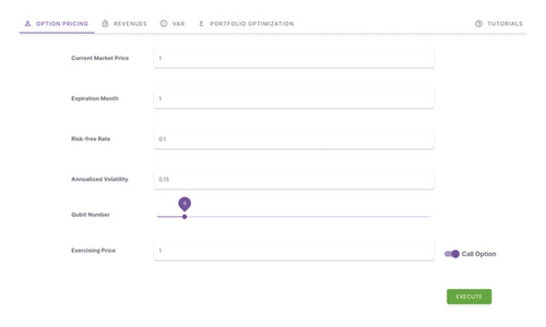
In the previous subsection, one see that quantum computing plays an important role in option pricing. However, for the general public, due to the mysteriousness of quantum computing itself, and it is neither easy nor practical to learn quantum computing and quantum programming. To overcome this problem, we have established a BQ-Bank web page, which provides software applications related to option pricing with a friendly user interface. We illustrate our modules for option pricing and option revenues with concrete examples.

(1) Option Pricing. The user interface for the quantum option pricing module of European-style is shown in Figure 1. In this user interface, we provide six main inputs as follows:

(1)
The current market price of the underlying asset
(2)
The option contract’s valid period
(3)
The risk-free interest rate
(4)
The annualized volatility
(5)
The option exercise price
(6)
The choosing option of call or put options

Details are in the caption following the image — **Figure 1**
Open in figure viewer PowerPoint

The user interface for the option pricing problem.

In the backend, we provide three algorithms to calculate the option price as follows:

(1)
Black–Scholes model
(2)
Quantum algorithm
(3)
Classic Monte Carlo algorithm

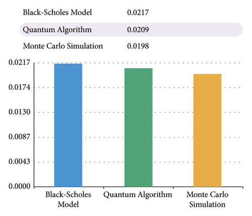
In conducting option pricing with the quantum algorithm, the users need to input the number of qubits (denoted with n) in the user interface. For the convenience of comparison, the sampling number of the classic Monte Carlo algorithm is set to 2ⁿ. After clicking the execution button, the calculation result is shown in Figure 2, with respect to the standard value shown by the Black–Scholes model, and the result of option pricing from the quantum algorithm is better than that from the classical Monte Carlo algorithm. Because of the randomness involved in both algorithms, the results will vary slightly from run to run.

(2) Option Revenues. Due to the discrepancy between the option price calculated by the theoretical model and the option price in the real market, speculators can arbitrage by buying and selling options. An application for calculating the expected option revenues strategy is also integrated into BQ-Bank, and the quantum algorithm in the backend is still based on the previous quantum option pricing algorithm. Specifically, this module calculates the expected option revenues portfolio by estimating the price of each option with a quantum option pricing algorithm and comparing it with the option market price.

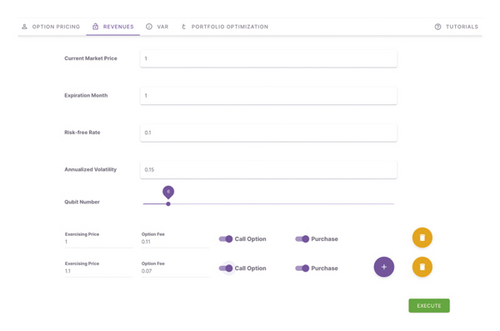
Similar to the inputs of option pricing, one can find the user interface for calculating expected option revenues in Figure 3. In addition to four inputs (i.e., the current market price of the underlying asset, the option contract’s valid period, the risk-free interest rate, and the annualized volatility of the asset), there are also other user input parameters required to construct an option portfolio. For example, to add another pattern of options by clicking the “+” sign icon at the end of its option input line, and to delete one pattern of options by clicking its respective “trash can” icon. Each pattern of options contains the option for call/put option, the option for buying/selling options, its exercising price and the option fee.

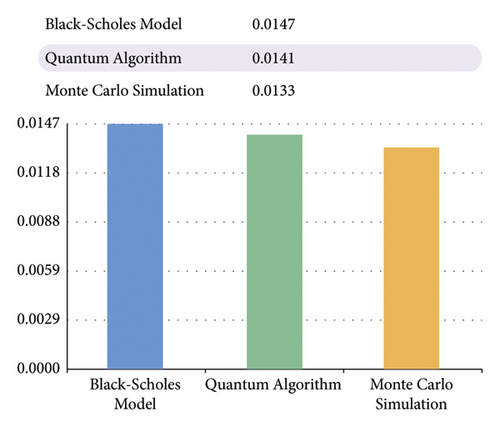
After executing the calculation, the result is shown in Figure 4. From the figure, we can get the estimated value of the expected revenues obtained by the three algorithms for the option portfolio we set. With respect to the standard value shown by the Black-Scholes model, the result with the quantum algorithm is better than the classical Monte Carlo algorithm’s. Also, due to the randomness involved in both algorithms, the results will vary slightly from run to run.

2.2. Value at Risk (VaR)

2.2.1. Classical Solution

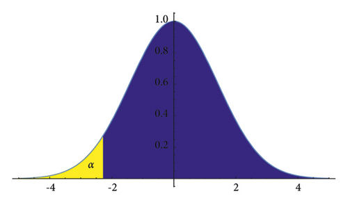
VaR is a parameter used to assess investment losses [19], and is often used as a risk measure of risk management. A more specific definition gives that the value of the maximum expected loss of an asset portfolio due to market price changes within a given confidence interval during the holding period, as depicted in Figure 5, takes the form of

()

where X is the profit and loss distribution (note the loss value is negative and the profit value is positive), α is the given probability, and F_X is its cumulative distribution function.

There are three kinds of classical VaR algorithms, namely, Historical VaR (H-VaR), Parametric VaR (P-VaR), Monte Carlo VaR (MC-VaR) [20]. However, these algorithms rely on different assumptions, so that their final VaR values are often different.

(1) H-VaR. When we have a certain amount of historical data in our hands but do not know the probability distribution of asset losses, we can assume that the asset’s future losses and gains are merely repetitions of past situations. Then, we use the VaR of the historical data to estimate the future VaR. The specific method is to sort the historical data by size, and determine the position of VaR in the sorting according to the product of the probability α and the size of the historical data.

(2) P-VaR. If we assume that the asset’s loss distribution follows a normal distribution, we can use historical data to estimate the mean and variance of the normal distribution, then use the normal distribution function to calculate the VaR at the probability α.

(3) MC-VaR. Here, we use the Monte Carlo method to simulate future asset market changes. A variety of risk factors need to be considered in the simulation process, which makes the simulation methods diverse and difficult. Among them, the geometric Brownian motion model is relatively simple. In the process of computer simulation, the geometric Brownian motion discrete model is

()

where S_t is the price of the asset at time t, ∆S_t is the first-order difference of the prices, μ is the mean value of historical returns, σ is the standard deviation of historical returns, and ∆t is the unit time of returns. In the MC-VaR method, we randomly select ϵ according to the normal distribution N(0,1) at each step of the time evolution of the asset holding period, so as to calculate sampling points on the expiration date.

2.2.2. Quantum Solution

In this subsection, we show how the QAE algorithm applies in calculating VaR [21, 22]. We discretize a random variable X and then map it into a qubit system {0,1,2, …, M − 1}, M = 2^m, where m is the number of sampled qubits, so any random variable X can be represented by a quantum state with probability p_i in state |i〉:

()

Consider a quantum operation F acting on sampling qubits and an ancillary qubit

()

where function f(i) ∈ [0,1]. Similar to (5), we can get the following equation:

()

Employing the QAE algorithm, we can obtain the quantum state probability with the ancillary qubit in state |1〉.

If we define function f(i) as

()

Equation (19) can be rewritten as

()

Thus, we can get the probability of the ancillary qubit in state |1〉, . When x ≤ k, there exists F_X(x ≤ k_α) ≥ α, which means k_α is the VaR with a confidence of α and a precision of O(M⁻¹), showing the quantum algorithm has a quadratic speedup compared to the classical MC-VaR method O(M^−1/2).

2.2.3. Examples and Results

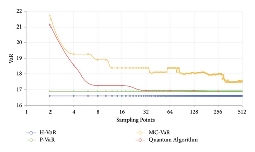
Now, we show how three different classical VaR algorithms, H-VaR, P-VaR, and MC-VaR, and our quantum algorithm perform for the same instance. As we can see, in the case studied in Figure 6, we choose the normal distribution as our model, 0.95 confidence and 30 holding days of assets which are combined of two assets, China Bao An and Ping An Bank with 10 of each are purchased.

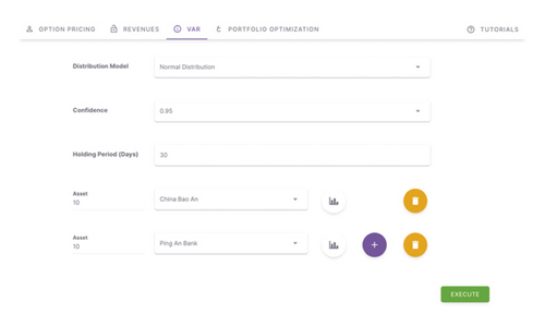
The results for both classical and quantum methods in different sampling points are shown in Figure 7, where we see that H-VaR and P-VaR are independent of the sampling points, which is quite intuitively obvious since both are calculated mainly based on historical data of assets without any sampling. As to MC-VaR, its VaR approaches to P-VaR with sampling points increasing, and even at 512 sampling points, there are still a small difference between P-VaR and MC-VaR. While the VaR with quantum algorithm approaches P-VaR monotonically with sampling points increasing and at 32 or larger sampling points, the VaR with the quantum algorithm is exactly equal to P-VaR. As the result shown in this instance, the VaR with the quantum algorithm is closer to P-VaR than that with the Monte Carlo method at the same sampling point, and we argue that the quantum algorithm performs better than the Monte Carlo method.

2.3. Portfolio Optimization

2.3.1. Model

Portfolio optimization [23] is an important problem that many investors will encounter. It requires investors to invest in candidate financial assets in order to minimize the risk under the condition of a certain return or maximize the investment return under the condition of a certain risk. If the number of candidate assets is very large, the classical algorithms used to solve such problems usually have high time complexity and are difficult to implement. Thanks to the powerful computing performance of quantum computing, the quantum algorithm can give the portfolio of assets with the optimal budget number among the candidate assets [24].

We use the mean-variance combinatorial optimization method, and the model for this problem can be expressed as

()

where

(i)
x ∈ {0,1}ⁿ in quantum algorithms represents the vector of binary decision variables. If the asset i is purchased, x_i = 1 and x_i = 0 when not. x_i ∈ [0,1] in classical algorithms is the weight of purchasing the corresponding asset, and ∑_ix_i = 1.
(ii)
represents the expected return of each asset.
(iii)
represents the covariance between the expected returns of each asset.
(iv)
q > 0 is the risk factor, which indicates the investor’s investment risk preference.
(v)
1 represents a n-dimensional vector whose elements are all 1 s.
(vi)
b represents the investment budget, which is the number of assets purchased from n assets in quantum algorithms case (assuming the price of each asset is 1). Usually, b = 1 in classical algorithms case.

2.3.2. Quantum Solution

According to the equation of the problem model in (22), the loss function is given as follows:

()

in which the first term represents the risk of the investment, the second term is the return of the investment, and the last term is a penalty function with A as the penalty parameter and is usually set large.

Our portfolio optimization scheme uses a combination strategy of classical and quantum methods. First, it uses quantum algorithms to select the optimal portfolio of assets with a budgeted number of n candidate assets. Then, it uses classical algorithms to calculate the assets selected by quantum algorithms (i.e., QAOA). Finally, it predicts the optimal strategy of purchasing assets and achieves maximum returns. With the aid of quantum algorithm, we can filter out the assets that do not need to be purchased, and the difficulty in implementing the classical algorithm is greatly reduced.

QAOA [25, 26], which can be classified as a variational quantum algorithm (VQA) [27, 28], is a quantum algorithm with a wide range of applications in the recent Noisy Intermediate-Scale Quantum (NISQ) [29] era. QAOA was proposed by Edward Farhi et al. in 2014 to approximately solve the combinatorial optimization problems. For a combinatorial optimization problem, which can be defined by a binary string of n bits z = z₁ … z_n, the aim is to determine the string that minimizes or maximizes the classical objective function .

QAOA can transform a combinatorial problem into an optimization problem. By mapping the binary variables into quantum spin operators

, the classical objective function can be changed into a quantum Hamiltonian:

()

whose ground state corresponds to the optimal solution of the problem.

In the case of QAOA with p layers, we usually initialize the state of the quantum system as |>+〉^⊗n and then alternately act the problem Hamiltonian H_C and the mixed Hamiltonian on the quantum system as follows:

()

which results in a wave function with 2p variational parameters as follows:

()

The expected value of H_C under this variational wave function can be obtained by measuring the quantum system:

()

then, solve the optimal parameter (γ^∗, β^∗) on a classical computer, achieving

()

In the ideal case, the quantum state |φ(γ^∗, β^∗)〉 should be the optimal solution, but it should be noted that the depth p of a parameterized quantum circuit is not infinite, so it is likely that

()

So, |φ(γ^∗, β^∗)〉 contains only the approximate optimal solution. Suppose |φ(γ^∗, β^∗)〉 is a superposition of l computational basis states, i.e.,

()

Usually, the greater of the probability that the ground state is measured in the eigenstate of H_c, the greater of the probability that its corresponding bit string e_i is the optimal solution.

2.3.3. Examples and Results

In conducting portfolio optimization with quantum algorithms, we made two assumptions about the problem to simplify the model:

(1)
All assets should have the same price (assumed to be 1)
(2)
The given budget should be an integral multiple of the price of an asset, and it needs to be all used for investment, which means that b assets need to be purchased

In this case, the portfolio optimization problem under these two assumptions corresponds to choosing a subset of b assets from n assets. We need to convert the loss function shown in (23) into a Hamiltonian to complete the encoding of the portfolio optimization problem. Because the value of the binary variable x_i (0 or 1) indicates whether the asset needs to be purchased, we need to construct a Hamiltonian whose eigenvalues corresponding to them. Since the eigenvalue of the Pauli operator σ^z is ±1, we can construct the Hamiltonian as , which corresponds to two eigenvalues 0 and 1. So, one can use the mapping to convert the loss function L_x into a Hamiltonian whose ground state corresponds to the optimal solution of the portfolio optimization problem.

As mentioned previously, we use a variational quantum algorithm, especially QAOA, to approximately solve the ground state of a Hamiltonian. Here, we list the procedure how we solve the portfolio optimization problem with QAOA and other algorithms:

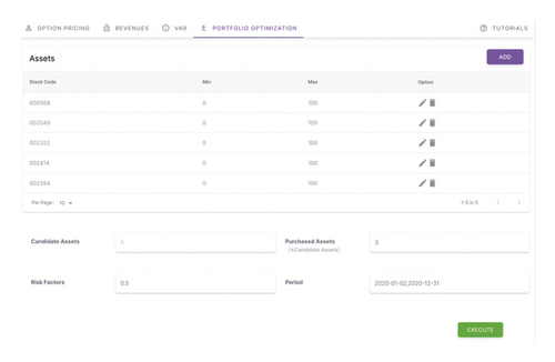
(1) Preparation. For each candidate asset x, given its preferred maximum share max_x and minimum share min_x (where max_x , min_x ∈ [0,1]) of the combinatorial assets, purchased assets budget b(b ⩽ n), risk factor q, and historical period of all candidate assets [t_i, t_f], as shown in Figure 8.

(2) Assignment. When the minimum share of an asset satisfies min_x > 0, it means the asset will definitely be purchased and will be assigned into the assets set X₁, and the total number of the assets set X₁ is defined as n₁. Else when min_x = 0, the asset needs to be determined by QAOA whether it needs to be purchased or not, and which asset will assigned into another assets set X₂.

(3) Optimal Selection with QAOA. Since there are already n₁ assets that have been determined to be purchased for sure, only (b − n₁) assets need to be selected from the set X₂ using QAOA. According to the mapping , the loss function L_x can be converted into a systematic Hamiltonian H_C with qubit number (n − n₁), and the ground state of this Hamiltonian is the optimal solution, where the mixing Hamiltonian is .

The following procedure is divided into two parts:

(i)
Quantum Part. Prepare a variational state |φ(θ, β)〉 = U(θ, β)| + 〉^⊗n on a quantum computer, where , and then obtain the expectation of Hamiltonian |φ(θ, β)〉 = U(θ, β)+〉^⊗n.
(ii)
Classical Part: Update θ, β with the classical optimization algorithm, such as COBYLA, and go back to the quantum part until λ approximately reaches a minimum. The optimal combination of assets to be purchased, as defined , is obtained from the variational state at this point, and the optimal combination of assets to be purchased is .

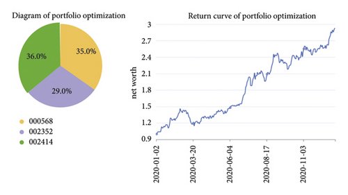
(4) Proportion Optimization. Finally, a trust-constr constraint algorithm is used to give the optimal proportion of the assets in the optimal portfolio to the constraints of every asset as assigned in the preparation step. Figure 9 shows the optimal result of an input example corresponding to Figure 8, including the optimal portfolio and its corresponding history return curve.

3. Summary

We have developed a quantum software BQ-Bank, which comprises 4 modules: option pricing, option revenues, VaR, and portfolio optimization. In each module, we start with the underlying problems and models, then we discuss the conventional algorithms and their quantum solution, and at the end we take an example and compare the results of the conventional algorithms with their quantum solution. The results show that the quantum solution usually outperforms the conventional algorithms. With the succinct design and the preset data set of BQ-Bank, people with or without quantum background can access and complete their interest tasks on a silver platter without trained skills.

Conflicts of Interest

The authors declare that they have no conflicts of interest.

Acknowledgments

The authors would like to thank Dr. Zai-sheng Lin for helpful discussions. This work was supported by the National Natural Science Foundation of China (Grant nos. 12004206 and 12005015).

Open Research

Data Availability

The data sets generated and/or analyzed during the current study are available from the corresponding author upon reasonable request.

Supporting Information

References

1 Paul B., The computer as a physical system: a microscopic quantum mechanical Hamiltonian model of computers as represented by turing machines, Journal of Statistical Physics. (1980) 22, no. 5, 563–591.
10.1007/BF01011339
Web of Science® Google Scholar
2 Feynman R. P., Simulating physics with computers, International Journal of Theoretical Physics. (1982) 21, no. 6/7.
10.1007/BF02650179
Web of Science® Google Scholar
3 Shor P. W., Algorithms for quantum computation: discrete logarithms and factoring, Proceedings of the 35th annual symposium on foundations of computer science, November 1994, Santa Fe, NM, USA, IEEE, 124–134.
Google Scholar
4 Grover L. K., Quantum mechanics helps in searching for a needle in a haystack, Physical Review Letters. (1997) 79, no. 2, 325–328, https://doi.org/10.1103/physrevlett.79.325, 2-s2.0-4243807288.
10.1103/PhysRevLett.79.325
CAS Web of Science® Google Scholar
5 Long G. L., Grover algorithm with zero theoretical failure rate, Physical Review A. (2001) 64, no. 2, 022307, https://doi.org/10.1103/physreva.64.022307, 2-s2.0-85037192799.
10.1103/PhysRevA.64.022307
Web of Science® Google Scholar
6 Harrow A. W., Hassidim A., and Lloyd S., Quantum algorithm for linear systems of equations, Physical Review Letters. (2009) 103, no. 15, 150502, https://doi.org/10.1103/physrevlett.103.150502, 2-s2.0-70349862042.
10.1103/PhysRevLett.103.150502
CAS PubMed Web of Science® Google Scholar
7 Orús R., Mugel S., and Lizaso E., Quantum computing for finance: overview and prospects, Reviews in Physics. (2019) 4, 100028, https://doi.org/10.1016/j.revip.2019.100028, 2-s2.0-85062038994.
10.1016/j.revip.2019.100028
Google Scholar
8 Tang H., Pal A., Wang T.-Yu, Qiao Lu-F., Gao J., and Jin X.-M., Quantum computation for pricing the collateralized debt obligations, Quantum Engineering. (2021) 3, no. 4, https://doi.org/10.1002/que2.84.
10.1002/que2.84
Google Scholar
9 Bachelier L., Théorie de la spéculation, Annales Scientifiques de l′Ecole Normale Superieure. (1900) 17, 21–86, https://doi.org/10.24033/asens.476.
10.24033/asens.476
Google Scholar
10 Cox J. C., Ross S. A., and Rubinstein M., Option pricing: a simplified approach, Journal of Financial Economics. (1979) 7, no. 3, 229–263, https://doi.org/10.1016/0304-405x(79)90015-1, 2-s2.0-49249142814.
10.1016/0304-405X(79)90015-1
Web of Science® Google Scholar
11 Rendleman R. J. and Bartter B. J., Two-state option pricing, The Journal of Finance. (1979) 34, no. 5, 1093–1110, https://doi.org/10.1111/j.1540-6261.1979.tb00058.x, 2-s2.0-84977406630.
10.1111/j.1540-6261.1979.tb00058.x
Web of Science® Google Scholar
12 Boyle P. P., A lattice framework for option pricing with two state variables, Journal of Financial and Quantitative Analysis. (1988) 23, no. 1, 1–12, https://doi.org/10.2307/2331019, 2-s2.0-84959674840.
10.2307/2331019
CAS PubMed Web of Science® Google Scholar
13 Black F. and Scholes M., The pricing of options and corporate liabilities, Journal of Political Economy. (1973) 81, no. 3, 637–654, https://doi.org/10.1086/260062.
10.1086/260062
Web of Science® Google Scholar
14 Brassard G., Hoyer P., Mosca M., and Tapp A., Quantum amplitude amplification and estimation, Contemporary Mathematics. (2002) 305, 53–74, https://doi.org/10.1090/conm/305/05215.
10.1090/conm/305/05215
Google Scholar
15 Suzuki Y., Uno S., Raymond R., Tanaka T., Onodera T., and Yamamoto N., Amplitude estimation without phase estimation, Quantum Information Processing. (2020) 19, no. 2, 75–17, https://doi.org/10.1007/s11128-019-2565-2.
10.1007/s11128-019-2565-2
Web of Science® Google Scholar
16 Scott A. and Rall P., Quantum approximate counting, simplified, Symposium on Simplicity in Algorithms, 2020, 24, SIAM, 32.
Google Scholar
17 Grinko D., Gacon J., Zoufal C., and Woerner S., Iterative quantum amplitude estimation, Npj Quantum Information. (2021) 7, no. 1, 52–56, https://doi.org/10.1038/s41534-021-00379-1.
10.1038/s41534-021-00379-1
Web of Science® Google Scholar
18 Zoufal C., Lucchi A., and Woerner S., Quantum generative adversarial networks for learning and loading random distributions, Npj Quantum Information. (2019) 5, no. 1, 103–109, https://doi.org/10.1038/s41534-019-0223-2.
10.1038/s41534-019-0223-2
Web of Science® Google Scholar
19 Yamai Y., Yoshiba T. et al., On the validity of value-at-risk: comparative analyses with expected shortfall, Monetary and Economic Studies. (2002) 20, no. 1, 57–85.
Google Scholar
20 Paul G., Heidelberger P., and Shahabuddin P., Efficient Monte Carlo methods for value-at-risk, Mastering Risk. (2000) 2, 5–18.
Google Scholar
21 Egger D. J., Garcia Gutierrez R., Mestre J. C., and Woerner S., Credit risk analysis using quantum computers, IEEE Transactions on Computers. (2021) 70, no. 12, 2136–2145, https://doi.org/10.1109/tc.2020.3038063.
10.1109/TC.2020.3038063
Web of Science® Google Scholar
22 Woerner S. and Egger D. J., Quantum risk analysis, Npj Quantum Information. (2019) 5, no. 1, 15–18, https://doi.org/10.1038/s41534-019-0130-6, 2-s2.0-85071911403.
10.1038/s41534-019-0130-6
Web of Science® Google Scholar
23 Durand D., Portfolio selection: efficient diversification of investments, The American Economic Review. (1960) 50, no. 1, 234–236.
Web of Science® Google Scholar
24 Nannicini G., Performance of hybrid quantum-classical variational heuristics for combinatorial optimization, Physical Review A. (2019) 99, no. 1, 013304, https://doi.org/10.1103/physreve.99.013304, 2-s2.0-85060180853.
10.1103/physreve.99.013304
CAS Web of Science® Google Scholar
25 Farhi E., Goldstone J., and Gutmann S., A quantum approximate optimization algorithm, 2014, https://arxiv.org/abs/1411.4028.
Google Scholar
26 Zhou L., Wang S. T., Choi S., Pichl2.1er H., and Lukin M. D., Quantum approximate optimization algorithm: performance, mechanism, and implementation on near-term devices, Physical Review X. (2020) 10, no. 2, 021067, https://doi.org/10.1103/physrevx.10.021067.
10.1103/PhysRevX.10.021067
CAS Web of Science® Google Scholar
27 Peruzzo A., McClean J., Shadbolt P., Yung M. H., Zhou X. Q, Love P. J., O’Brien J. L., and Aspuru-Guzik A., A variational eigenvalue solver on a photonic quantum processor, Nature Communications. (2014) 5, no. 1, 4213–4217, https://doi.org/10.1038/ncomms5213, 2-s2.0-84904819361.
10.1038/ncomms5213
CAS PubMed Web of Science® Google Scholar
28 Moll N., Barkoutsos P., Bishop L. S., Chow J. M., Cross A., Egger D. J., Filipp S., Fuhrer A., Gambetta J. M., Ganzhorn M., Kandala A., Mezzacapo A., Muller P., Riess W., Salis G., Smolin J., Tavernelli I., and Temme K., Quantum optimization using variational algorithms on near-term quantum devices, Quantum Science and Technology. (2018) 3, no. 3, 030503, https://doi.org/10.1088/2058-9565/aab822, 2-s2.0-85049985621.
10.1088/2058-9565/aab822
Web of Science® Google Scholar
29 Brooks M., Beyond quantum supremacy: the hunt for useful quantum computers, Nature. (2019) 574, no. 7776, 19–21, https://doi.org/10.1038/d41586-019-02936-3, 2-s2.0-85072927620.
10.1038/d41586-019-02936-3
CAS PubMed Google Scholar

Citing Literature

All articles

BQ-Bank: A Quantum Software for Finance and Banking

Abstract

1. Introduction