The purpose of this paper is to carry out an alternative to the present transient models for field wound synchronous machines, which is able to take into account the nonlinearity of the magnetic materials as well as the cross-magnetization. After presenting the principal model structures according to the state variables, a model based on two lookup tables for the magnetizing flux linkages is introduced and built step by step. The resulting signal flowchart shows an algebraic loop within the model, where the main flux linkage rapidly converges to its instantaneous value by simple iteration. The proof of this convergence is given for both saturated and unsaturated machine. Even though the proposed model uses the total linkage flux as state variable, as many alternative models do, it does not require the inversion of the current to flux linkage function (i.e., of lookup tables). This can spare a heavy computational task, especially with very large lookup tables. In the proposed model, the computational effort in the worst case scenario is reduced to few iterations (<10). Finally, the nonlinear behavior of the model is verified in four different transient scenarios by comparing its outcomes with those of a linear model for the same test machine.

1. Introduction

The study of synchronous machines (SM) in nonstationary behavior has taken advantage of the Park theory since many decades. The separation of the combined actions of all machine magnetomotive forces (MMFs) along the two electrically orthogonal rotor magnetic axes makes the corresponding magnetic flux linkages independent from the relative position between rotor and stator. This simplifies in turn the solution of the electromechanical differential equations (DEs) which describe the machine behavior, since the machine self-inductance and mutual inductance become time invariant. Nevertheless, the nonlinearity of the magnetic properties prevents the problem to be simply solved by the theory of linear DE or the Laplace transform. Therefore, the numerical integration of DE by means of computational resources has become the main way to simulate SM-related transient phenomena making use of a d-q axis model. Transient related to the electric system dynamic stability [1, 2], symmetrical and asymmetrical faults [3, 4], load rejection [5], and asynchronous behaviors [6–8] have done large use of nonlinear SM models based on the d-q axis theory. In more recent time, the interest for the transient model of SMs has been awaken by the applications of embedded systems (ES) to the control of SM for industrial and traction applications [9–13]. In that case, the model is used in the observer of a driven motor, in order to predict its state variables. In this specific task, the model must fulfil not only the usual requirement to be accurate in the predictions but also to deliver them quickly. This fact well represents the observer dilemma between the complexity of the model on one side and the need for its computational lightness on the other side. For example, taking into account the nonlinearity and the cross-magnetization introduced by the ferromagnetic materials in a SM model [14, 15], it improves the outcome accuracy of the model itself, but it requires more computational resources. In order to tackle this computational problem, lookup tables (LUTs) [14, 16] are increasingly preferred to analytic formulas [17, 18] for implementing the nonlinearity and the cross-magnetization in SM models. In fact, LUTs can provide the armature flux linkage for a given magnetomotive force (MMF) just by entering a multidimensional numerical table and picking up its value. All that without getting the CPU involved in any sort of time-consuming calculation. Nonetheless, for the experimental and the computational determinations of the relationship between the flux leakages and the currents, see the currents as sources and the linked fluxes as outcomes [16, 17]. For this reason, the flux-linkage-to-current LUT, which is needed in the model using the flux linkage as state variable, cannot be measured or calculated straightforwardly. It must rather be obtained through the inversion of the current-to-flux-linkage function Ψ(i). In an ingenious closed loop [14, 16], control strategies have been invented, which are nested in a numeric iterative procedure, in order to obtain the flux-linkage-to-current LUT moving from an available current-to-flux-linkage one. Besides, the recourse to a SM model having the current as variable of state, which makes knowingly use of the straight function Ψ(i), does not lighten the calculation burden anyway, since a marginal inductance matrix l(i) of the machine and its inversion are also needed [17]. This paper offers a solution for using a SM machine transient model having all machine flux linkages as state variables, without any need for the inversion of the current-to-flux-linkage LUTs. The key idea for bypassing the issue of the Ψ(i) inversion is the recourse to LUTs which are related to the magnetizing flux linkages along the d-axis and the q-axis rather than to the whole flux linkages. Then, the machine currents can be alternatively obtained from the distance vector between the flux linkages and the main fluxes via a constant leakage matrix, which is related to the machine stray inductances. Therefore, particular attention is paid in this paper to the construction of the leakage matrix starting from the most suitable and general SM model. Moreover, provided an input for the machine state of magnetization together with the external electrical and mechanical constraints at a given time, it is proved that the proposed model converges necessarily to the instantaneous values of the state variables. In the part dedicated to the method, after having revised the possible structures for a SM model and introduced a complete SM d- q-axis model, the paper shows the linear proportionality between the machine currents and the distance vector between main and flux linkages. Hence, the alternative flux linkage-based model is built, and its convergence to the timely state variables is demonstrated. The model is tested on a 60 kVA, 400 V, 50 Hz salient pole synchronous machine (SPSM). The method for obtaining the related LUTs by means of FEM calculations is described in the appendix, whereas the implications of the nonlinearity and the cross-magnetization on the machine behavior are discussed in the paper body. The section dedicated to the results shows the simulations obtained by means of the novel model. Four different transitory behaviors have been simulated: (1) rapid transition from nominal excitation to underexcitation and back; (2) 10% sudden increase of the grid voltage; (3) rapid drop of the driving torque (-75%) under constant power factor; and (4) severe voltage sag (-60%) lasting several cycles. The results achieved through the proposed model are compared with the ones achieved for the same SPSM by a linear model (i.e., having constant d-axis and q-axis magnetizing inductances) in order to highlight the errors introduced in the results by neglecting nonlinearity- and cross-magnetization-related phenomena in the machine model.

2. Materials and Methods

2.1. A Novel Structure for the SM Model

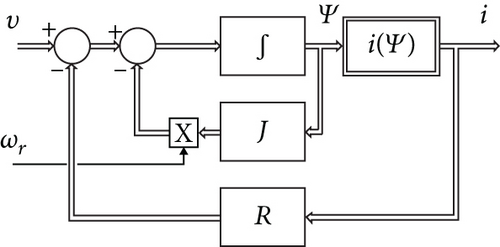
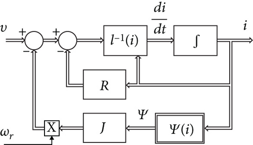
In [19], it has been proved that by assuming the SM flux linkages or alternatively the currents as state variables, or even considering a combination of them, several different SM equivalent models can be obtained. Nevertheless, in the practical applications, the most recurrent models [17] are those represented in Figure 1. In particular, the model in Figure 1(a) assumes the armature flux linkage vector Ψ as a state variable whereas the model in Figure 1(b) uses the armature currents vector i to that end. The last model is straightforwardly apt to host a LUT that relates the flux linkage vector to the armature currents. In fact, as soon as the machine is considered anhysteretic, the function Ψ(i) becomes single-valued. Hence, it can be univocally approximated, in a domain D of the armature currents, by interpolating a finite number of its samples collected in a LUT. Since the anhysteretic assumption has the collateral drawback of disregarding part of the magnetic losses in the machine, they need to be reintroduced into the model later on. Fortunately, there are many available methods [9] for doing that, and this specific topic will therefore not be dealt in the present paper.

Details are in the caption following the image — **Figure 1 (a)**
Open in figure viewer PowerPoint

Typical structures of a SM model having (a) the flux linkage or (b) the current as a variable of state.

However, choosing the current vector as a state variable procures additional complexity to the model: the construction of the incremental inductance matrix

()

on one side and the calculation of its inverse l⁻¹ on the other side. Both [16, 17] agree in preferring the model of Figure 1(a) to that of Figure 1(b) because it leads to more simple state equations. Moreover, in ES making use of a full order observer, the flux linkage vector is always available. Conversely, if the observer does not have full rank, the model of Figure 2(b) must be forcibly used according to the state of the art, due to the lack of estimations for the flux linkages.

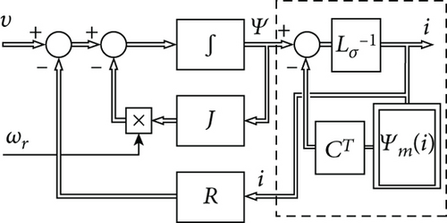
The novel model proposed by the present work is represented in Figure 2.

The following can be observed: (I) it keeps all flux linkages, not only those of the armature, as state variables; (II) it implements the function i(Ψ) of Figure 1(a) by combining a constant matrix , to be yet defined, and a nonlinear single-valued function Ψ_m(i), which represents the armature main flux linkages. Feature (I) spares the use of (1) in the model as well as the issue of its inversion, whereas feature (II) introduces the novelty of the suggested model. In particular, it does not require the construction of the inverse function i(Ψ) starting from Ψ(i) as shown in [14, 16], and it is applicable to reduced order observers as well, since its saturation model Ψ_m(i) works upon available current measurement/estimation rather than on flux linkage ones.

However, the exploitation of this model requires two aspects to be clarified in advance. First of all, the machine currents are a linear combination of flux linkages and magnetizing flux linkages according to

()

with

and C being the constant matrices to be defined. Second, the block diagram within the shaded box in Figure 2 forms an algebraic loop, which sets a convergence problem in a discrete time integration of the related DEs. At the generic integration instant t_k, the highlighted block gets the estimated vector of the flux linkages Ψ_k as an input. Two possible outcomes can occur within the next time instant t_k+1: either the generic main fluxes Ψ_m,j converge to their actual values at t_k—providing through that an estimation for the currents i_k at the same time—or they diverge making the simulation progress impossible. From a system perspective, the proof of the convergence within the loop is equivalent to demonstrate the existence of a solution i in

()

for all possible Ψ, once the main flux Ψ_m(i) is expressed by means of LUTs

()

where

()

2.2. Stray Flux Linkages vs. Current Proportionality

A quite general Park model for a wound field salient pole synchronous machine (SPSM) is represented in Figure 3, where two armature circuits (outside the shaded circle) and three rotor circuits (inside the shaded circle) are considered. In particular, with reference to the rotor, there are the excitation circuit (f) and a single damper circuit (D) on the d-axis and a single damper circuit (Q) on the q-axis.

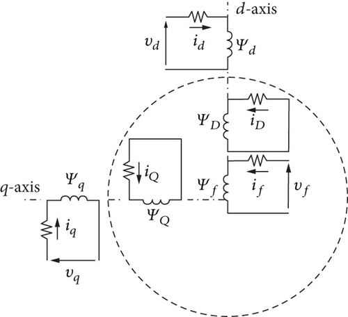
A more precise consideration of a round rotor SM (RRSM) would have required two more rotor circuits on both axes indeed: one for taking into account the presence of the massive and conductive rotor body and the other one for the eventual conductive slot wedges. In the same way, the consideration of a permanent magnet excited SM (PMSM) should replace the excitation winding in Figure 3 with a suitable and permanent source of MMF, in order to fit in the representation. Nevertheless, the circuits of Figure 3 are general enough for presenting the proposed model in its entirety.

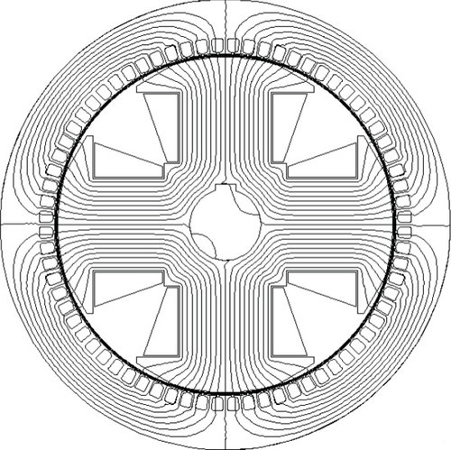
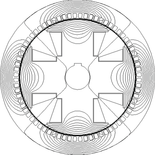
The more simplistic assumption often done about the Park model of Figure 3 is that the circuits along the d-axis share all the same magnetizing flux. In other words, their mutual inductances referred to the armature side are considered all equal to the main armature inductance on the d-axis, L_md

()

Canay [20], Hiramatsu et al. [21], and Guorui et al. [22] have proved that (6) does not always hold. Not only the main fluxes but also the stray fluxes contribute to the mutual linkage between the circuits laying on the same magnetic axis. Figure 4(a) shows, e.g., that the magnetic coupling between the excitation winding and the D-damper bars in a RRSM takes place through the stray fluxes too. In fact, all rotor circuits, excitation winding and damper bars, are usually laid down in the same slots.

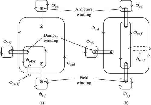
In this way, the main flux Φ_mDf, shared between excitation winding and D-damper bars, becomes larger than Φ_md, i.e., the flux they have in common with the armature. In a SPSM having grid-shaped damper bars on each pole, a part Φ_σaf of the magnetic flux Φ_maf—produced by the armature and linked to the field winding—does not link the D-damper bars. Therefore, Figure 4(b) shows that the flux Φ_md linking the D-damper circuit can be smaller than the flux Φ_maf shared between the armature and the excitation winding. The practical consequence of these remarks is the introduction of an additional stray inductance in the usual Park model as shown in Figure 5. It takes into account the algebraic difference between the total main flux, which links the armature on the d-axis, and the total flux shared between field winding and D-damper circuit.

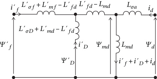
According to the observations presented above, it results that can be negative for SPSM while it is always positive for RRSM.

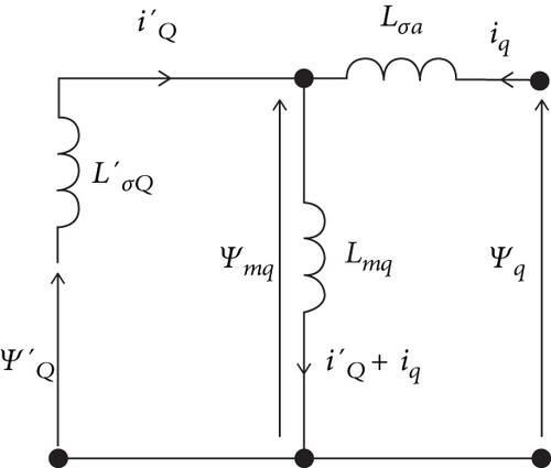
Since the circuits along the q-axis in Figure 3 are only two, there is just one quadrature main flux to be considered. Therefore, the equivalent magnetic circuit on the q-axis looks like the one represented in Figure 6.

Having the circuits of Figures 5 and 6 under consideration at once, the following relationship can be set between the currents and the flux linkages at play.

()

all quantities used in (7) being referred to the armature side. Hence, the inverse of the 5 × 5 matrix L_σ, called the matrix of the stray inductance, takes the form

()

where

()

The Blondel coefficient was introduced:

(i)
Stray coefficient for the armature
()

Laible’s coefficients are as follows [23]:

(i)
Stray coefficient between armature and field winding
()
(ii)
Stray coefficient between armature and D-damper circuit
()
(iii)
Stray coefficient between armature and field winding
()
(iv)
Stray coefficient between armature and Q-damper circuit
()
(v)
Armature shielding coefficient
()
(vi)
Field winding shielding coefficient
()
(vii)
D-damper circuit shielding coefficient
()
as well as the machine anisotropy factor at nominal conditions
()

The inverse matrix of the stray inductances ((8)) turns into

()

In (19),

represents the armature direct axis inductance at nominal conditions and

()

When studying (10)–(17) closer, it can be recognized that the stray and the shielding coefficients can be regarded as constants. In fact, they represent ratios where numerators and denominators vary according to the same underlying nonlinear magnetization characteristics, irrespective to d-axis or q-axis consideration. Adding that and AF^N are also constants, it can be concluded that (19) is a constant matrix and that (7) sets a linear proportionality between the vector of the stray fluxes and the vector of the machine currents.

2.3. Variable Convergence within the Algebraic Loop

The armature main flux linkages on the d- and q-axes depend on the superposed action of all MMFs at work on the d- and q-axes, respectively. Once the currents of the rotor circuits have been referred to the armature side, they are armature currents at all effects, so that the sources of the main fluxes can be summarized as follows:

()

with

()

A more concise expression for (7) can be written by using (22).

()

which, once substituted in (21), takes the form

()

For later considerations, it is here anticipated that

()

where

()

When considered in relative terms, (26) and (27) become

()

By considering the discrete values of (5) as one possible choice among the ∞² sets of values generated by the magnetizing flux functions

and

, it is possible to generalize (5) as

()

so that the inverse of (30)

()

exists locally in D⁻¹ as soon as

()

By considering (21), (24), and (31) at the same time, it is possible to obtain

()

Equation (33) sets a Banach fixed point problem, where the numerical sequence

()

converges to a finite value

()

if and only if, ϕ represents a contracting map of D⁻¹ towards D or simply when

()

The function ϕ^′ stands for the Jacobian of ϕ. Since Ψ is kept constant during the eventual convergence in (33), the Jacobian of ϕ has the following expression:

()

Due to (32) the function Ψ_m can be inverted, so that (37) turns into

()

Finally, taking into account (25), (30), and (38), the inequality (36) changes into

()

where l_m,dd, l_m,dq, and l_m,qq are the elements of the symmetric matrix l_m accounting for the incremental magnetizing inductances of the SM.

By making use of (39), it is possible to give a proof of the studied convergence (35) within the algebraic loop of the proposed SM model, for both the nonsaturated and saturated machines. In fact, when the SM is not saturated, the incremental inductances (which stand for the slopes of the tangents to the magnetizing curves on the d- and q-axes, respectively) are comparable with the magnetizing inductances (which stand for the slopes of the chords from the origin to the magnetizing curves along the d- and q-axes, respectively). In other terms,

()

Moreover, the lack of saturation, i.e., the availability of plenty of nonoriented Weiss domains in the SM magnetic circuit, makes the competition for the magnetic polarization between the coordinated MMFs practically inexistent. That means

()

Taking into account (10) and substituting (40) and (41) in (39) lead to the inequality

()

Expression (42) fulfils condition (36) for the convergence. In fact, even assuming an unrealistically large armature stray inductance of about 30%, the d-axis inductance should be at least 10 times larger than the q-axis one in order to have >1.

If the SM is saturated instead, any further differential increase of the coordinated MMFs will not gain any new Weiss domain to their respective directions, so that the incremental magnetizations contributed by the MMFs can be regarded as essentially performed in air. For the same reason, the magnetic anisotropy of the machine fades away making AF≅1. Therefore,

()

At the same time, the lack of available domains to compete for inhibits the mutual coupling between the coordinated circuits through the cross-magnetization. This results in

()

By substituting (43) and (44) in (39), the fulfilment of (32) for the case of the machine saturation is also achieved, since

()

Due to the local monotonic nature of the magnetization functions (30), it must be expected the transition from (42) to (45) to be also monotonic, to ensure the convergence (35) for every simulated machine behavior between saturation and nonsaturation.

2.4. Model Implementation

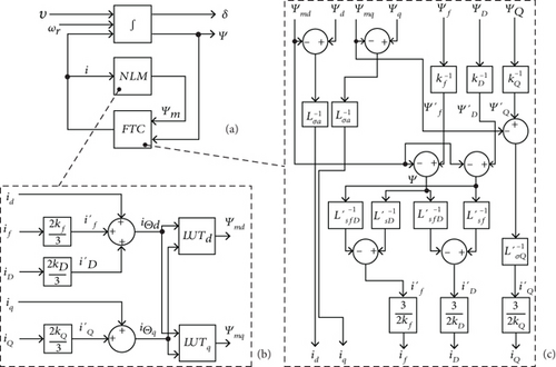
The model presented in Figure 2 has been implemented by means of three functional blocks shown in Figure 7(a). The block performing the integration is the same used in the state of the art and presented in Figures 1(a) and 1(b). It has essentially the goal to gain the state variable Ψ by integrating the unbalances between the impressed voltages, the resistive voltage drops, and the transformational electromotive forces, where present. The nonlinearity manager (NLM) block, in Figure 7(b), receives the current vector as an input and refers the rotor currents to the armature side by making use of the following transformation ratios:

()

The transformed currents, which provide their MMFs on the same d- or q-axes, are summed up in order to determine the armature equivalent magnetizing currents and , respectively. The LUT_d reproduces the function shown in Figure 8(a), whereas LUT_q reproduces the shown in Figure 8(b). One possible way to build the lookup tables for a given SM by using a FEM analysis program is duly described in the appendix to the present work.

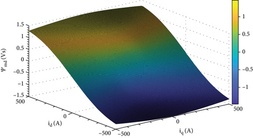
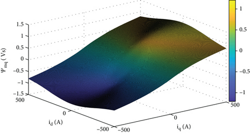
As soon as the coordinated magnetizing current is introduced in the LUTs, two values for the armature main flux linkages are returned as outputs, Ψ_md and Ψ_mq, respectively.

These quantities provide the inputs for the flux-to-current (FTC) block in Figure 7(c) together with the vector of the flux linkages Ψ. The rotor-related flux linkages must be referred to the armature side by means of the ratios (46). Then, as already shown in (7), the block performs a linear combination of the linked stray fluxes through the matrix , in order to get an estimate of the machine currents. The currents obtained by that way are all referred to the armature side. Therefore, the rotor-related currents need to be referred back to the rotor by using the usual ratios (46).

2.5. Performed Test Simulations

The proposed nonlinear model for SM has been tested on the wound field SPSM (WFSPSM) shown in Figure 9, the parameters of which are given in Table 1.

Table 1. Main parameters of the test SM.

Symbol	Description	Value
A_N	Rated power	60 kVA
V_N	Rated voltage	400 V
n_N	Rated speed	1500 rpm
f_N	Rated frequency	50 Hz
cos φ_N	Rated power factor	0.9
δ_min ⋯ δ_max	Airgap range at the pole shoe	3.2 ÷ 5.7 mm
α_p	Pole coverage	0.76
l_i	Active axial length	184 mm
r_δ	Airgap average radius	161 mm
q	Slots per pole per phase	6
n_s	Conductors per slot	8
r	Armature phase resistance (p.u.)	6.2 · 10⁻²
r_f	Field winding resistance (p.u.)	5.8 · 10⁻³
r_D	d-axis damp. circuit resistance (p.u.)	7.7 · 10⁻³
r_Q	q-axis damp. circuit resistance (p.u.)	15.3 · 10⁻³
	Nominal d-axis reactance (p.u.)	1.32
	Nominal q-axis reactance (p.u.)	0.72
AF^N	Nominal anisotropy factor	0.83
σ_a	Armature stray factor	5.2%
σ_af	Field winding to armature stray factor	9.7%
σ_aD	Armature to d-axis damper circuit stray factor	11.8%
σ_Q	q-axis damper circuit stray factor	13.3%
μ_a	Armature shielding coefficient	1.7%
μ_f	Field winding shielding coefficient	9.5%
μ_D	q-axis damper circuit shielding coefficient	11.7%

In order to prove the capability of the suggested model in handling the nonlinearity and the cross-magnetization in the test machine, the model itself has been compared with a linear and anisotropic one, where the LUTs of Figure 7(b) have been replaced by constant magnetizing inductances L_md and L_mq. The latter has been chosen, for each led test, so as to match the initial conditions of the nonlinear model, before an external cause intervenes to push the machine away from its initial steady state. In this way, the two models are aligned at the beginning of the test, and all subsequent divergences between them can be recognized more clearly. In particular, four tests have been envisaged, that, for the nature of the chosen perturbation, end up changing the magnetizing flux and highlighting the magnetic nonlinearity of the machine.

The first test foresees the sudden drop of the excitation voltage from its nominal value down to 40% of it, while the nominal driving torque of the generator is kept constant. Therefore, the generated nominal active power remains unchanged. Due to the lack of exciting MMF, the machine must require the magnetizing current from the grid, moving by that from the generation to the consumption of reactive power.

The second test is based on the observation that the voltage level at the generator bus bar is responsible for the incoming/outgoing reactive power. Therefore, a grid voltage increase, when the excitation current is kept constant, results in a higher magnetizing flux in the SM. This should in turn shift the generator towards the saturation and possibly highlight its underlying nonlinear behavior.

The third test reproduces the adjustment of the excitation current when the generated power is suddenly reduced down to 25% of its nominal value. In order to keep the power factor constant, the excitation current is decreased accordingly, so that the exciting MMF is drastically reduced.

The fourth and final simulations deal with a low-voltage fault ride through (LVFRT), where the grid voltage experiences a severe sag, like the one (class 3) foreseen for the industrial environment, in the reference standard for EMC tests EN61000-4-34. By increasing the duration of the sag, the stability limit for the SM is detected. The comparison between the limits—achieved through the linear and nonlinear model, respectively—should show to what extent the nonlinear magnetization matters in modelling stability problems.

3. Results and Discussion

3.1. Excitation Voltage Step Test

Figure 10 shows the instantaneous drop of the SM excitation voltage, at the time t = 3 s, in the test machine providing the nominal power at the nominal conditions. This change in the control voltage produces a subsequent and slower drop of the excitation current.

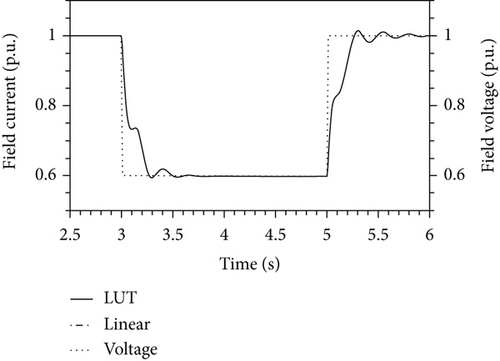
It is not possible to observe any substantial difference between the resulting field currents for the nonlinear and linear model, since the d-damper bars screen the field winding from the large variations of the armature MMFs occurring during the transient. Figure 11 shows that the d-axis component of the armature current drops almost to zero whereas the q-axis one increases.

Since the electromagnetic torque remains unchanged, from the Park equation for the torque follows that

()

where Ψ_d, at steady state and for i_d≅0, is

()

In Figure 11, it is possible to observe that |i_q| in the linear model is larger than that in the nonlinear one. Since the excitation current

is the same for the two models (Figure 10), by considering (47) and (48), it follows

()

where

()

because of

()

By remembering that the magnetizing inductances of the linear model are kept constant and equal to the initial magnetizing inductances of the nonlinear model, from (50) descends

()

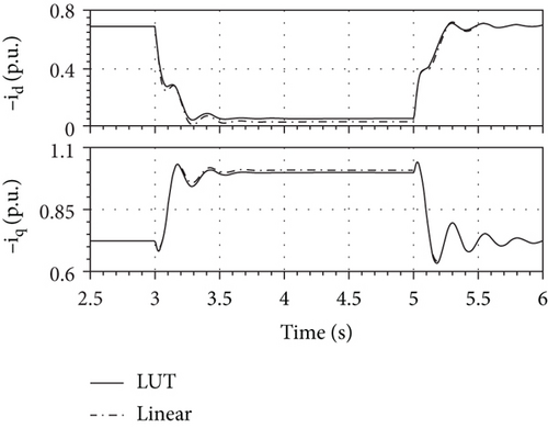
Inequality (52) proves that the magnetizing inductance of the nonlinear model senses the transition from the over excitation to the under excitation, since its value increases when the magnetizing flux decreases. The transition from the over excitation to the under excitation is given also from the graph of the reactive power in Figure 12.

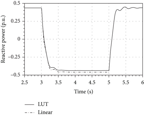
The SM produces reactive power as long as the rotor MMF is strong enough. As soon as the excitation current drops, the generator starts consuming reactive power. It can also be observed that, since i_d≅0,

()

The larger value of the |i_q| in the linear model observed in (51) together with (53) explains the discrepancy between the answers of the two models shown in Figure 12.

3.2. Grid Voltage Step Test

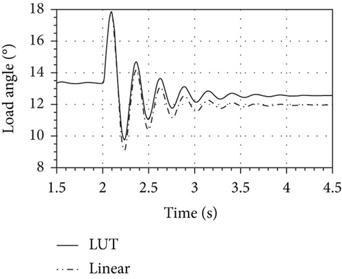
In this test, while the generator is providing 60% of the nominal power at cos φ = 0.9 (lagging), a stepwise 10% increase of the grid voltage occurs at t = 2 s. In Figure 13, it can be observed that the two models give a different account of the d-axis and q-axis currents in the final steady state, as well as of the generator load angle, as it is shown in Figure 14. In particular, Figure 14 shows, firstly, that the load angle δ decreases moving from the initial steady state to the final one and, secondly, that the linear model provides a smaller load angle for the final steady state, δ_lin, than the one given by the nonlinear model, δ_LUT.

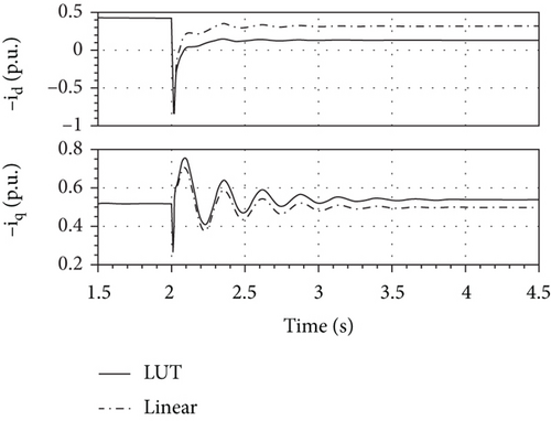
Moreover, since the excitation of the SM and its driving torque are kept constant, the generated active power does not change when the transient response fades away, whereas the reactive power does (Figure 15). The nonlinear model gives account of a drop in the reactive power provided by the generator, which is larger than the one reported by the linear model.

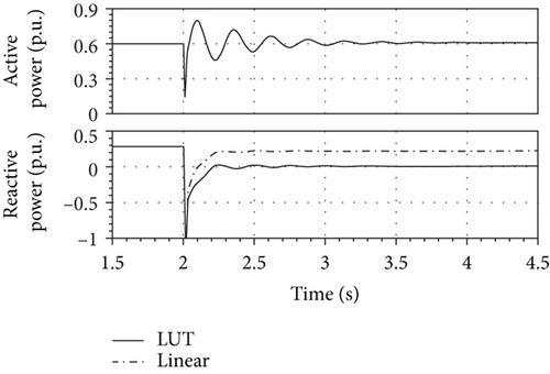
Figure 16 helps to interpret and check the different results shown in Figures 14 and 15.

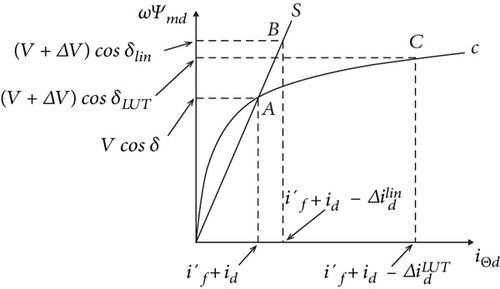
The letter A indicates the magnetic work point shared by the two models at the initial steady state, when the same q-axis voltage sets the same magnetizing flux linkage on the d-axis according to

()

In (54), the voltage drop on the armature stray inductance is neglected, since it is irrelevant to the present line of reasoning.

At the initial work point A, the main flux linkage is set by the superposition of the MMF proportional to

and i_d, respectively. As soon as the grid voltage is incremented by ΔV > 0, the magnetic flux linkage in the linear model increases up to

()

due to 0 < δ_lin < δ in Figure 14. Since the model is linear, the MMF responsible for Ψ_md(B) can be found by the vertical projection of the point B on the x-axis, which is taken on the straight s at y = ωΨ_md(B). It can be observed that the resulting MMF corresponding to the work point B gives a correct account of a drop of the direct axis current in the final steady state, since

for graphic construction.

Coming to the nonlinear model in Figure 16, an increase ΔV > 0 of the grid voltage produces an increase of the magnetic flux linkage up to

()

due to 0 < δ_LUT < δ in Figure 14. At the same time, it must be

()

due to 0 < δ_lin < δ_LUT in Figure 14. The MMF, which sets Ψ_md(C), can be determined by the vertical projection of the point C on the x-axis, which is taken on the nonlinear magnetization curve c in Figure 16 at y = ωΨ_md(C). It can be noticed that the resulting MMF corresponding to the work point C gives a correct account of a drop in the direct axis current for the final steady state, since

. Moreover, the graphic construction shows that

in spite of (57), just in reason of the magnetic nonlinearity of the SM taken into account in the model containing the LUTs. The much stronger reduction of the i_d in the nonlinear model rather than in the linear one is the reason of the opposite tendency of the i_q in the two models, shown in Figure 13. In fact, the constant machine torque during this test

()

sets a relationship between i_d and i_q. The small decrease of the i_d in the linear model does not change the torque effectively whereas the i_q is forced to decrease in order to compensate the relevant linear increase in Ψ_md. On the contrary, in the nonlinear model, the drop in i_d is substantial, and due to the small increase of the main flux linkage Ψ_md, the i_q must be larger than in the linear model for keeping the torque constant.

3.3. Driving Torque Step Test (at Constant Power Factor)

The present test foresees a driving torque drop from 100% down to 25% of its nominal value within 0.1 s. At the same time, in order to target the same initial power factor (0.9 lagging) in the final steady state, the excitation current is decreased accordingly. Figure 17(a) shows the needed adjustments of the field current whereas Figure 17(b) and the generated active power.

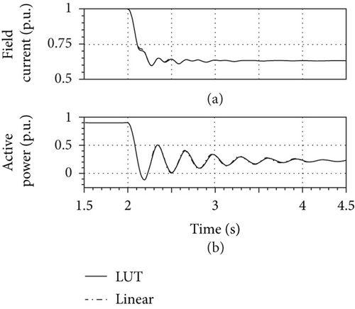
Even though Figure 17 does not present relevant differences between the answers of the two models, in Figure 18, they give a different account for the envelope of the armature phase current amplitude.

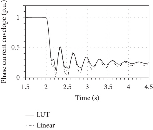
The mismatch between the two answers depends mainly on the direct axis current, as Figure 19 reveals by showing the different steady-state values for the reactive power.

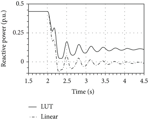
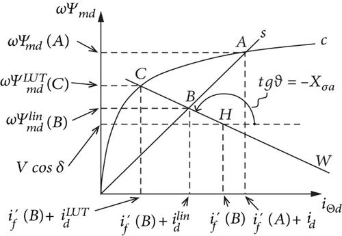
The difference between the values of the i_d in the two-models can be justified by the Park armature voltage equation along the q-axis at steady state, where the d-axis current is given by

()

Since the load angle δ decreases due to the drastic drop of the generated active power, so that cosδ≅1, the Ψ_md plays the main role in producing the difference between the two steady-state values of i_d provided by the models. Figure 20 shows how the magnetic work point in the linear model moves from A to B along the straight s, until the main flux Ψ_md(B) is set through the constant magnetizing inductance and the superposed effects of the currents and .

Equation (59) shows that for ωΨ_md to exactly balance the quadrature axis voltage at i_d = 0, the main flux Ψ_md must be set by

only. This is way, by following the straight w (having slope −ωL_σa) down to the point H at y = Vcosδ, it is possible to find the current

. Since the final value of the excitation current

and the quadrature axis voltage Vcosδ is shared by the two models, by prolonging w up to the nonlinear magnetization characteristic c, the final magnetic work point C for the nonlinear model is found. By comparing the points C and B, it can be recognized that

()

which gives a right account of the nonlinear property of the SM magnetic circuit. Furthermore, it can be found that

()

which explains why neglecting the nonlinearity in the SM model would lead to underestimating the value of the reactive power provided at low excitation.

3.4. Low-Voltage Fault Ride Through

In the following last test, two voltage sags with the same intensity (-60% of the nominal grid voltage) but different duration (14 and 18 cycles, respectively) are applied to the armature of the SM. The response of the generator is simulated by means of the two models under comparison. This test, which evaluates the capability of the SM to keep the pace when the disturbance is over, represents a LVFRT test. Figure 21 shows that both machines keep the pace for a sag duration of 14 cycles. No substantial differences between the final steady-state values of the load angle can be recognized.

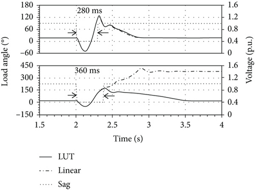
In the same figure, for a duration of the sag of 18 cycles, the nonlinear model proves the SM to be able to keep the pace after the sag, whereas the linear model does not.

The different results provided by the two models can be interpreted in an intuitive way through the application of the well-known equivalent area criterion, as shown in Figure 22. In there, the difference between the constant driving torque T_m and the electromagnetic torque T is responsible for the acceleration work on the rotor. The electromagnetic torque can be expressed by

()

where

and

are the transient reactances of the SM along the d- and q-axes, respectively. Since the transient reactances are related to the stator and rotor stray inductances essentially, the nonlinearity of the magnetic circuit does not influence their values in a substantial way. Therefore, the different performances of the two models must be caused by their different transient electromotive force E^′. In particular, in order to justify the results of Figure 21, it must be true that, during the voltage sag,

()

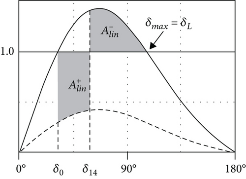
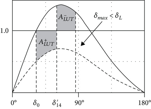
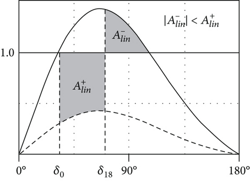
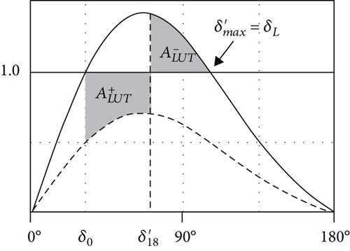
In studying Figure 22, it emerges that the nonlinearity of the SM magnetic circuit confers to the machine itself, a given capability to withstand grid voltage sags. Neglecting the said nonlinearity in the SM model leads to underestimating the machine performances during LVFRT tests.

3.5. Anisotropy and Cross-Magnetization: 1 or 2 LUT?

A relevant question considers the possibility of using just one single LUT instead of two for expressing both anisotropy and cross-magnetization in the SM. In that case, the LUT_d related to Ψ_md could be used in first place. In order to obtain Ψ_mq from LUT_d, its values should be scaled down, e.g., by a suitable constant which depends on the anisotropy factor AF. As long as the LUT_d represents a function of i_d and i_q, some information about the influence of the q-axis MMF on the cross-magnetization must be contained in LUT_d. In fact, some energy considerations presented in [15, 24] make it possible to infer that

()

Therefore, as soon as

()

it is evident that identity (64) is violated, because, from (65), it follows

()

Hence, it seems impossible to give a correct account of the cross-magnetization by using the information coming from just one single LUT.

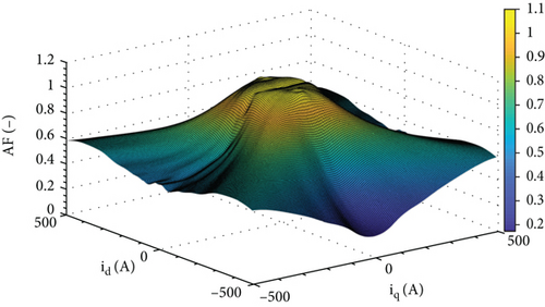
With reference to the anisotropy factor AF instead, in many works, the ratio between L_d and L_q is kept constant, even though it proves to be strongly dependent on the intensities of i_d and i_q and on their relative ratio. In Figure 23, the AF_m (see the appendix for its definition) for the test SM of Figure 9 has been represented. It gives an evidence of the fact that the anisotropy of a SM is in general not constant. It tends to fade away for very deep saturation, since the magnetic circuit reluctance along the d- and q-axes becomes comparable in magnitude. Even more important is the fact that the cross-magnetization contributes to foster the anisotropy of the machine. It is possible to observe this fact in Figure 23, where the anisotropy factor shows higher values along two crossed versants, which run along the 1^st to 3^rd and 2^nd to 4^thi_d-i_q quadrant directions. This is probably due to the competing action of the coordinated MMFs on the material polarization, which prevents one axis to reach the full saturation when the other one is excited at the same time.

3.6. An Estimate for the Convergence Speed of the Algebraic Loop in the Model

Equation (33) represents a contracting map ϕ(D)⟶D when the SM iron is unsaturated (42) as well as when it is not (43). Therefore, it is possible to calculate the number k (in excess) of the needed iterations in order to get

close enough to its asymptotic value

, according to a given relative accuracy ε. With M representing the upper bound of the Jacobian ϕ^′ over D, it results as follows:

()

After calculating the upper bound M_sat = 0.351 in (45) by means of (28) and (29), the maximal number of iterations (67) reducing the initial error about one thousand times (ε = 10⁻³) is k = 7.

4. Conclusions

A two-axis theory-based SM model has been presented, which takes into account the nonlinearity of the SM magnetic circuit as well as the cross-magnetization. These performances are achieved by using two LUTs that reproduce the magnetizing flux linkages of the machine armature. Following this authors’ choice, the outlined model does not need any inversion of the current-to-flux-linkage LUT, even if the model maintains the flux linkages as state variables. This is possible thanks to a LUT-centered algebraic loop, which is intrinsic into the model and whose iterations always converge to the instantaneous machine main flux. The proof for the convergence of the introduced algebraic loop has been given for both cases of nonsaturated and saturated machines. The novel SM model has been successfully tested for the simulation of a wholly specified salient pole synchronous generator. Four different transient scenarios have been considered, where as many external disturbances provoke a substantial perturbation on the machine main fluxes, so to highlight the magnetic nonlinearity at play in the model. The outcomes have been compared with those of a traditional linear Park model for the same SM, giving a punctual interpretation and explanation of the occurred discrepancies.

All tests performed have shown that neglecting the nonlinearity of the machine magnetization characteristic leads to remarkable divergences between the two model outcomes. Finally, the construction of the main flux linkages LUTs for the test SM has highlighted the importance of a correct account of the machine magnetic anisotropy. In particular, the assumption of a constant ratio between the d-axis and q-axis armature inductances cannot be representative of all machine behaviors. In fact, the anisotropy of the SM depends not only on the absolute values of the direct and quadrature armature currents but also on their ratio. Moreover, it has been found out that the cross-magnetization leaves a recognizable signature on the machine magnetic anisotropy profile and that this fact cannot be reproduced by using one single LUT in the model. For all exposed reasons, the authors believe that the proposed model can be of a certain interest for those who perform simulations of SM in classic power systems applications, as well as in the control tasks of the modern electric drives. In this last field, this model can be used in reduced order observers, since its underlying mechanism for reproducing the magnetic nonlinearity relies on the use of the measured currents rather than on the flux linkages.

Symbols

i:: Current vector
i_d:: d-axis component of the armature voltage
i_q:: q-axis component of the armature voltage
i_D:: Current in the d-axis rotor damper circuit
i_Q:: Current in the q-axis rotor damper circuit
i_f:: Excitation current
I:: Rotor moment of inertia
J:: Cross-matrix for the stator motional EMFs
l:: Matrix of the marginal inductances
l_m:: Matrix of the marginal magnetizing inductances
:: Inverse Matrix of the stray inductances
:: Field winding stray inductance seen from the armature
:: Field winding main inductance seen from the armature
:: Direct axis damper circuit stray inductance seen from the armature
:: Direct axis damper circuit main inductance seen from the armature
:: Mutual inductance between the direct axis damper-circuit and the field winding
:: Mutual inductance between the armature and the field winding
:: Mutual inductance between the direct axis damper-circuit and armature
L_md:: Main or magnetizing direct axis inductance
:: Q-circuit stray inductance seen from the armature
R:: Park-matrix of the resistances
v:: Voltage vector
v_d:: d-axis component of the armature voltage
v_q:: q-axis component of the armature voltage
v_f:: Excitation voltage
Ψ:: Flux linkage vector
Ψ_m:: Main flux linkage vector
Ψ_d:: d-axis armature flux linkage
Ψ_q:: q-axis armature flux linkage
Ψ_md:: d-axis magnetizing flux linkage
Ψ_mq:: q-axis magnetizing flux linkage
:: D-damper circuit flux linkage seen from the armature
:: Q-damper circuit flux linkage seen from the armature
:: Field winding flux linkage seen from the armature
ω_r:: Rotor angular speed.

Disclosure

The research presented in this paper was carried out as a part of “Swedish Hydropower Centre (SVC).”

Conflicts of Interest

The authors declare that there is no conflict of interest regarding the publication of this paper.

Acknowledgments

SVC has been established by the Swedish Energy Agency, Energiforsk and Svenska Kraftnät together with Luleå University of Technology, KTH Royal Institute of Technology, Chalmers University of Technology, Uppsala University, and the Faculty of Engineering at Lund University. Participating companies and industry associations are as follows: AFRY, Andritz Hydro, Boliden, Fortum Sverige, Holmen Energi, Jämtkraft, Jönköping Energi, Karlstads Energi, LKAB, Mälarenergi, Norconsult, Rainpower, Skellefteå Kraft, Sollefteåforsens, Statkraft Sverige, Sweco Sverige, Tekniska verken i Linköping, Uniper, Vattenfall R&D, Vattenfall Vattenkraft, Voith Hydro, WSP Sverige, and Zinkgruvan.

Appendix

In Figures 5 and 6, it can be observed that the main fluxes on the two magnetic axes are set by the superposition of the d-axis and q-axis MMFs, respectively. Once the currents are all referred to the armature side, they can be easily added one another, without distinguishing anymore which one of them and in what measure contributes to the magnetization or demagnetization of the machine. This makes it possible to determine the current-to-magnetizing-flux characteristics by using only the armature currents. In fact, once the ranges for the d-axis and q-axis armature currents have been chosen, a convex and closed domain D is defined as follows:

()

The domain D(i_d, i_q) ϵ ℝ² corresponds univocally to the domain T(i_a, i_b, i_c) ϵ ℝ³ of the machine phase currents by means of the 3 × 2 reduced Park matrix P.

()

where the zero sequence component has been disregarded

()

As soon as the d-axis is aligned with the electric axis a of the armature phase A (which means pϑ = 2kπ for k = 0, 1, 2, ⋯), the reduced matrix P turns into the reduced Clarke matrix, so that

()

If the DC currents i_a, i_b, and i_c of (A.4) supply the phases, A, B, and C of a SM, respectively, a radial flux density B_n will be established in the machine airgap. It depends on the electric angle pα measured starting from the electrical axis a of the phase A. The spatial harmonics of the flux density in phase with cos(kpα) are those contributing to the main flux linkage along the d-axis. In the same way, the flux density harmonics in phase with sin(kpα) are those producing the main flux linkage along the q-axis. Hence, the fundamental coordinated main flux linkages can be determined by

()

where

()

For SMs working as generators, where the EMFs are forcibly made pretty much sinusoidal through specific design choices, it is possible to consider the fundamental of the flux density only in (A.9) and (A.10), so that

()

One way for populating the LUTs by using the values of (A.11) and (A.12) is that of obtaining the radial flux density distribution B_n(pα) of the SM by a FEM calculation. The latter is nested in a loop which provides the phase currents (A.4) to the FEM program, which are needed for supplying the armature. In this way, the resulting magnetizing flux linkages Ψ_md and Ψ_mq are univocally related to the ordered pairs of i_d and i_q, respectively.

Once the magnetizing fluxes (A.11) and (A.12) are obtained, it is possible to yield the respective magnetizing inductances as follows:

()

Finally, the magnetic anisotropy factor AF_m for the SM is obtained by

()

Open Research

Data Availability

The data that support the findings of this study are available from the corresponding author upon reasonable request.

References

1 Hamidifar S. and Kar N. C., A novel approach to saturation characteristics modeling and its impact on synchronous machine transient stability analysis, IEEE Transactions on Energy Conversion. (2012) 27, no. 1, 139–150, https://doi.org/10.1109/TEC.2011.2176128, 2-s2.0-84857364023.
10.1109/TEC.2011.2176128
Web of Science® Google Scholar
2 IEEE guide for synchronous generator modeling practices and parameter verification with applications in power system stability analyses, IEEE Std 1110-2019, 2020, 1–92.
Google Scholar
3 Saha S. and Aldeen M., Dynamic modeling of power systems experiencing faults in transmission/distribution networks, IEEE Transactions on Power Systems. (2015) 30, no. 5, 2349–2363, https://doi.org/10.1109/TPWRS.2014.2365809, 2-s2.0-85027940486.
10.1109/TPWRS.2014.2365809
Web of Science® Google Scholar
4 Samanfar A., Shakarami M. R., Soltani J., and Rokrok E., Dynamic analysis of multi-machine multi-UPFC power systems experiencing transient asymmetrical faults, IET Generation, Transmission & Distribution. (2019) 13, no. 19, 4491–4502, https://doi.org/10.1049/iet-gtd.2018.6075, 2-s2.0-85073698477.
10.1049/iet-gtd.2018.6075
Web of Science® Google Scholar
5 Hiramatsu D., Uemura Y., Uemoto S., Okumoto J., Imai T., Kakiuchi M., Nagakura K., Fujita M., and Otaka T., Influence of quadrature-axis reactance of large turbine generator on operation, Electrical Engineering in Japan. (2011) 177, no. 3, 17–27, https://doi.org/10.1002/eej.21099, 2-s2.0-79960531280.
10.1002/eej.21099
Web of Science® Google Scholar
6 Hiramatsu D., Koyanagi K., Hirayama K., Uemura Y., Kakiuchi M., Satoh T., and Ara A., Study of asynchronizing phenomena using generator model with field mutual leakage reactance, Electrical Engineering in Japan. (2005) 153, no. 3, 31–40, https://doi.org/10.1002/eej.20147, 2-s2.0-25444504822.
10.1002/eej.20147
Web of Science® Google Scholar
7 Campeanu A., Enache S., Vlad I., and Enache M., Operation in asynchronous overload of synchronous motor. Effect of damping windings, 5th International Symposium on Electrical and Electronics Engineering (ISEEE), October 2017, Galati, Romania, 1–6.
Google Scholar
8 Deleanu S., Iordache M., Niculae D., Stanculescu M., Dogaru M., and Galan N., Dynamic operation of high power synchronous generator in asynchronous regime or encountering three-phase shortcircuit, 2018 International Conference on Applied and Theoretical Electricity (ICATE), 2018, Craiova, Romania, 1–8.
Google Scholar
9 Peretti L., Sandulescu P., and Zanuso G., Self-commissioning of flux linkage curves of synchronous reluctance machines in quasi-standstill condition, IET Electric Power Applications. (2015) 9, no. 9, 642–651, https://doi.org/10.1049/iet-epa.2015.0070, 2-s2.0-84947346617.
10.1049/iet-epa.2015.0070
Web of Science® Google Scholar
10 Calleja C., López-de-Heredia A., Gaztañaga H., Aldasoro L., and Nieva T., Validation of a modified direct-self control strategy for PMSM in railway-traction applications, IEEE Transactions on Industrial Electronics. (2016) 63, no. 8, 5143–5155, https://doi.org/10.1109/TIE.2016.2572661, 2-s2.0-84978914820.
10.1109/TIE.2016.2572661
Web of Science® Google Scholar
11 Tang Z., Li X., Dusmez S., and Akin B., A new V/f-based sensorless MTPA control for IPMSM drives, IEEE Transactions on Power Electronics. (2016) 31, no. 6, 4400–4415, https://doi.org/10.1109/TPEL.2015.2470177, 2-s2.0-84962407518.
10.1109/TPEL.2015.2470177
Web of Science® Google Scholar
12 Therrien F., Chapariha M., and Jatskevich J., Constant-parameter synchronous machine model including main flux saturation, IET Electric Power Applications. (2016) 10, no. 6, 477–487, https://doi.org/10.1049/iet-epa.2015.0447, 2-s2.0-84977112051.
10.1049/iet-epa.2015.0447
Web of Science® Google Scholar
13 Foo G. H. B. and Zhang X., Robust direct torque control of synchronous reluctance motor drives in the field-weakening region, IEEE Transactions on Power Electronics. (2017) 32, no. 2, 1289–1298, https://doi.org/10.1109/TPEL.2016.2542241, 2-s2.0-84999143030.
10.1109/TPEL.2016.2542241
Web of Science® Google Scholar
14 Chedot L. and Friedrich G., A cross saturation model for interior permanent magnet synchronous machine. Application to a starter-generator, Conference Record of the 2004 IEEE Industry Applications Conference, 2004. 39th IAS Annual Meeting, 2004, Seattle, WA, U.S.A, 64–70.
Google Scholar
15 Mingardi D., Morandin M., Bolognani S., and Bianchi N., On the proprieties of the differential cross-saturation inductance in synchronous machines, IEEE Transactions on Industrial Applications. (2017) 53, no. 2, 991–1000, https://doi.org/10.1109/TIA.2016.2622220, 2-s2.0-85017584722.
10.1109/TIA.2016.2622220
CAS Web of Science® Google Scholar
16 Antonello R., Peretti L., Tinazzi F., and Zigliotto M., Self-commissioning calculation of dynamic models for synchronous machines with magnetic saturation using flux as state variable, The Journal of Engineering. (2019) 2019, no. 17, 3609–3613, https://doi.org/10.1049/joe.2018.8259.
10.1049/joe.2018.8259
Web of Science® Google Scholar
17 Qu Z., Tuovinen T., and Hinkkanen M., Inclusion of magnetic saturation in dynamic models of synchronous reluctance motors, 2012 XXth International Conference on Electrical Machines, 2012, Marseille, France, 994–1000.
Google Scholar
18 Woo T.-G., Park S.-W., Choi S., Lee H. J., and Yoon Y. D., Flux saturation model including Cross Saturation for synchronous reluctance machines and its identification method at standstill, IEEE Transactions on Industrial Electronics. (2023) 70, no. 3, 2318–2328, https://doi.org/10.1109/TIE.2022.3174233.
10.1109/TIE.2022.3174233
Web of Science® Google Scholar
19 Rehaoulia H., Henao H., and Capolino G. A., Modeling of synchronous machines with magnetic saturation, Electric Power Systems Research. (2007) 77, no. 5–6, 652–659, https://doi.org/10.1016/j.epsr.2006.06.003, 2-s2.0-33846576638.
10.1016/j.epsr.2006.06.003
Web of Science® Google Scholar
20 Canay I. M., Causes of discrepancies on calculation of rotor quantities and exact equivalent diagrams of the synchronous machine, IEEE Transactions on Power Apparatus and Systems. (1969) PAS-88, no. 7, 1114–1120, https://doi.org/10.1109/TPAS.1969.292512, 2-s2.0-84938452262.
10.1109/TPAS.1969.292512
Web of Science® Google Scholar
21 Hiramatsu D., Koyanagi K., Hirayama K., Uemura Y., Kakiuchi M., Satoh T., and Nagasaka K., Estimation of field mutual leakage reactance in synchronous machine by line-to-line sudden short circuit test, IEEE Power Engineering Society General Meeting. (2004) 2, 1359–1366.
Google Scholar
22 Guorui X., Hongyu W., Xiaofang L., and Jinping K., The study about the precision of standard parameter models of synchronous machine, 2011 International Conference on Electrical Machines and Systems, 2011, Beijing, China, 1–5.
Google Scholar
23 Laible T., Die Theorie der Synchronmaschine im nicht-stationären Betrieb, 1952, Springer-Verlag.
10.1007/978-3-662-26051-7
Google Scholar
24 Melkebeek J. A. and Willems J. L., Reciprocity relations for the mutual inductances between orthogonal axis windings in saturated salient-pole machines, IEEE Transactions on Industrial Applications. (1990) 26, no. 1, 107–114, https://doi.org/10.1109/28.52681, 2-s2.0-0025211582.
10.1109/28.52681
Web of Science® Google Scholar

Citing Literature

All articles

A Synchronous Machine Transient Model Based upon an Algebraic Loop Accounting for Nonlinearity and Cross-Magnetization

Abstract

1. Introduction

2. Materials and Methods

2.1. A Novel Structure for the SM Model

2.2. Stray Flux Linkages vs. Current Proportionality

2.3. Variable Convergence within the Algebraic Loop

2.4. Model Implementation

2.5. Performed Test Simulations

3. Results and Discussion

3.1. Excitation Voltage Step Test

3.2. Grid Voltage Step Test

3.3. Driving Torque Step Test (at Constant Power Factor)

3.4. Low-Voltage Fault Ride Through

3.5. Anisotropy and Cross-Magnetization: 1 or 2 LUT?

3.6. An Estimate for the Convergence Speed of the Algebraic Loop in the Model

4. Conclusions

Symbols

Disclosure

Conflicts of Interest

Acknowledgments

Appendix

Open Research

Data Availability

References

Citing Literature

Figures

References

Information

About Wiley Online Library

Help & Support

Opportunities

Connect with Wiley

A Synchronous Machine Transient Model Based upon an Algebraic Loop Accounting for Nonlinearity and Cross-Magnetization

Abstract

1. Introduction

2. Materials and Methods

2.1. A Novel Structure for the SM Model

2.2. Stray Flux Linkages vs. Current Proportionality

2.3. Variable Convergence within the Algebraic Loop

2.4. Model Implementation

2.5. Performed Test Simulations

3. Results and Discussion

3.1. Excitation Voltage Step Test

3.2. Grid Voltage Step Test

3.3. Driving Torque Step Test (at Constant Power Factor)

3.4. Low-Voltage Fault Ride Through

3.5. Anisotropy and Cross-Magnetization: 1 or 2 LUT?

3.6. An Estimate for the Convergence Speed of the Algebraic Loop in the Model

4. Conclusions

Symbols

Disclosure

Conflicts of Interest

Acknowledgments

Appendix

Open Research

Data Availability

References

Citing Literature

Figures

References

Related

Information