1. Introduction

Acquiring accurate and reliable device parameters is crucial in the context of power distribution networks (PDNs) due to their multifaceted implications [1]. However, the lack of in situ measurement techniques poses challenges in directly obtaining certain PDN parameters, which are typically assumed to be static in real situations. These parameters include line resistance, line reactance, transformer resistance, transformer reactance, transformer conductance, and transformer electrical susceptance. This limitation often leads to poor estimation in parameter identification for PDN [2]. To address these challenges, numerous approaches have been developed to enhance numerical efficiency and reduce residuals in parameter estimation. These approaches include supervisory control and data acquisition, power management unit (PMU), and advanced metering infrastructure. They can be classified into various methods, such as the full-scale approach [3], PSOSR [4], normalized Lagrange multiplier (NLM) test [5], finite-time algorithm (FTA) [6], residual method, sensitivity analysis method, Lagrange multiplier method [7], Heffron-Phillips method [8], and specialized Newton–Raphson iteration [9]. Additionally, recent advancements in machine learning and deep learning techniques have led to the proposal of smart methods, including artificial neural network [10], graph convolution network (GCN) [11], support vector machine (SVM) [12], multihead attention network [13], deep reinforcement learning [14], estimation using synchrophasor data [15], PSCAD simulation [16], multimodal long short-term memory deep learning [17], and edge computing [18]. While these methods show effectiveness with simulation data, they often require specialized measuring devices.

To overcome the challenges posed by the lack of required data and measuring devices, a mathematical approach called the power flow model can be employed. The power flow model establishes relationships between PDN parameters and easily obtainable data, such as active power, reactive power, and voltage. The challenging parameters mentioned earlier can be optimized using algorithms in combination with the static parameters, namely, active power, reactive power, and voltage, on the low-voltage side. By utilizing the power flow model, the voltage values on the high-voltage side can be calculated, and the residuals between the calculated and true values can be used to construct a loss function for optimization methods. The optimization methods for parameter identification can be generally classified into two categories, namely, the gradient-free methods [19–25] and gradient-based methods [26, 27]. First, in gradient-free methods, the heuristic or biomimetic optimization rules are designed such as particle swarm optimization (PSO), genetic algorithm (GA), ant colony algorithm, Aquila optimizer (AO) [28], nuclear reaction optimization (NRO) [29], and Pareto-like sequential sampling heuristic method (PSS) [30]. The performance of these heuristic algorithms is largely dependent on the initialization. On the other hand, the gradient-based method is usually constructed by combining the physical model of PDN and the neural network with the backward propagation of the loss function. Beneficial from the chain rule and automatic derivative of the loss function with respect to the parameters to be optimized, the gradient-based method is a deterministic approach. Therefore, many advanced gradient descent algorithms can be utilized to accelerate the optimization. In addition, researchers pay more attention to data preprocessing methods, including the utilization of clustering algorithms and hypothesis testing [31, 32].

This paper is organized as follows. Section 2 introduces the identification equations of power flow model in PDN and proposes the AGBO-Pro optimization method. The experimental data and calculation details are given in Section 3. The results and discussions are given in Section 4. Finally, Section 5 gives a brief conclusion.

2. Materials and Methods

2.1. Power Flow Model Calculation

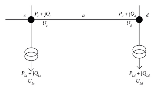
The fundamental principles of PDN analysis can be found in references [20, 31–33]. To streamline the computational process, the assumption of balanced three-phase condition is made as a prerequisite for power flow calculations in this work. The schematic diagram of power flow calculation circuit model is shown in Figure 1.

In Figure 1, P_d, Q_d, and U_d represent the active power, reactive power, and voltage on the high-voltage side of the transformers at bus D, respectively. These three parameters can be obtained directly by real-time measurements. Other parameters, such as transformer electrical R_d, transformer resistance X_d, transformer conductance G_d, transformer electrical susceptance B_d, line resistance R_cd, and line reactance X_cd, are in general hard to be detected in PDN calculation and satisfy the following equations:

$$ (1)

$$ (2)

$$ (3)

where $$ and $$ in equation (3) are the longitudinal and transverse components of the transformer impedance voltage drop at bus D. P_Ld, Q_Ld, and U_Ld represent the active power, reaction power, and voltage on the low-voltage side of the transformers at bus D, respectively. $$ and $$ can be obtained by the following equations:

$$ (4)

$$ (5)

The equation of bus C can be expressed as equations (6)–(8):

$$ (6)

$$ (7)

$$ (8)

where $$ and $$ in equation (6) are the longitudinal and transverse components of the transformer impedance voltage drop at bus C.

2.2. Theoretical Framework of AGBO-Pro for Parameter Identification in PDN

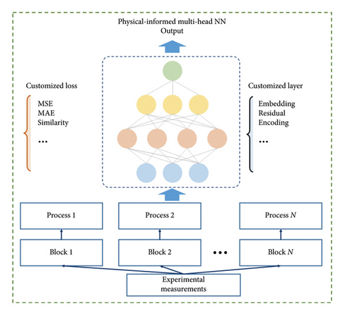
The schematic diagram is shown in Figure 2, where it is combined with gradient-based neural network (NN) and gradient-free optimization method. The inputs of the framework are experimental measurements of PDN, which can be divided into several blocks (or fields) including numerical features and categorical features. Each block can be processed via a customized way and then connected with customized layers. The loss function for gradient-based optimization is also flexible.

2.2.1. Physical-Informed Multihead Neural Network

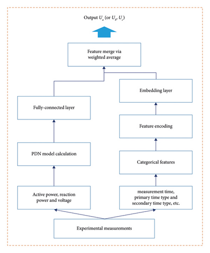
The experimental measurements of PDN can be classified into two categories, namely, the continuous (or numerical) features and discrete (or categorical) features such as measurement time, primary time type, and secondary time type. The numerical and categorical features are processed with different treatments by introducing a multihead neural network, which is shown in Figure 3. It is shown that the input layer of NN is separated into two blocks; the first includes numerical features, which are defined as X₁ = (P_Ld,i, Q_Ld,i, U_Ld,i) representing the set of the active power, reaction power, and voltage on the high-voltage side of the transformers, and the subscript i represents the sample points for i = (1,2, ⋯, N). The other includes categorical features X₂ = (T_i, P_i, S_i⋯), whereT_i and PV_irepresent the measurement and peak-valley period, respectively. It is noted that the recording duration has 24 categories, and the peak-valley electricity has 3 categories (i.e., high, medium, and low).

After the input layer of NN, the numerical features X₁ are fed into the PDN model, while the categorical features are first encoded (i.e., one-hot encoding) and then imported into an embedding layer to transform the sparse feature matrix into a dense matrix. After the embedding layer, we utilize the max-min normalization to scale the categorical features into ω₁ = [ω_1,0, ω_1,2, ⋯, ω_1,i] ∈ [0,1], which can be seen as a probability distribution. Then, the numerical and categorical features are merged with a linear combination as follows:

$$ (9)

where η represents the noise term, which is subject to the normal distribution, i.e., η ~ N(0,1). With the help of maximum likelihood estimation, the loss function of this work is defined as

$$ (10)

where y_i and $$ represent the theoretical calculation value of PDN and true value by experimental measurement, respectively. In addition, to avoid gradient vanishing during the backward propagation of NN, a nonlinear transformation, namely, sigmoid activation function rather than linear rectification function (ReLU), is utilized:

$$ (11)

Therefore, the loss function is further modified as

$$ (12)

where $$ represents the true value of voltage on the high-voltage side.

The above loss function is also known as the Euclidean distance measuring the difference between theoretical calculation and experimental observation. In this work, we also utilize a Pearson correlation loss function, which is defined as

$$ (13)

In the previous work, we have derived the gradients of the loss function with respect to R_d, X_d, G_d, B_d, R_cd, and X_cd. According to the PDN model, the loss function can be calculated with forward calculation; then, the back propagation of the gradient of the loss function can be applied to update the connection weight in NN.

2.2.2. Gradient-Based Optimization Algorithm

Once we have the above gradients of the loss function with respect to the parameters, then the gradient-based optimization can be implemented. The pseudocode of optimization method of this work is shown in Algorithm 1.

Algorithm 1: Adaptive gradient-based optimization methods.
•  

  Input: θ₀ initial parameters

•  

   f(θ) objective function to be optimized

•  

   β₁, β₂ decay rates for moment estimates

•  

   m₀ initialized first-order moment

•  

   υ₀ initialized second-order moment

•  

   t time step

•  

   η learning rate

•  

   l_∞  ←  2/(1 − β₂) − 1 maximum length of the simple moving average

•  

  While θ_t is not converged do

•  

   t  ←  t + 1

•  

   g_t  ←  ∇_θf_t(θ_t−1) gradient with respect to parameters at time step t

•  

   $$ update first-order moment

•  

   $$ update second-order moment

•  

   $$ biased-corrected first-order moment

•  

   $$ the length of the moving average

•  

   If the variance is tractable, i.e., l_t > 4then

•  

    $$ update the adaptive learning rate

•  

    $$ the variance rectification term

•  

    $$ update parameters

•  

   Else

•  

    $$

•  

  End while

•  

  Return θ_t

3. Dataset and Calculation Details

3.1. Data Collection and Description

In this work, a dataset including 1499 samples is collected via SCADA [33, 34] for the training of the proposed model. The voltage profiles on the high-voltage (U_a, U_b, and U_c) and low-voltage (u_a, u_b, and u_c) sides are presented in Figures 4 and 5, respectively.

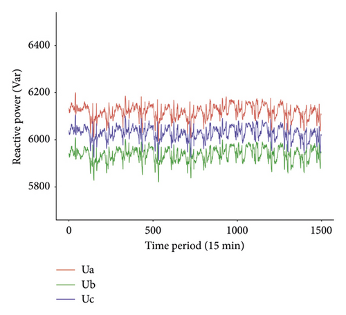
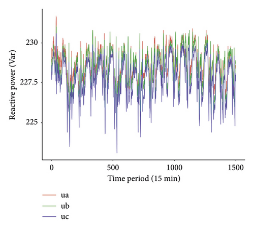
From Figures 4 and 5, it is found that the high-voltage sides in the dataset are similar to the three-phase balance satisfying the equations in Section 2.1. In addition, the active power (P_a, P_b, and P_c) and reactive power (Q_a, Q_b, and Q_c) profiles on the low-voltage side are given in Figures 6 and 7, respectively.

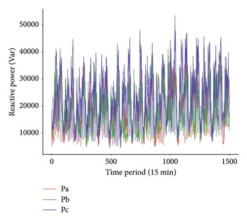
It is found from Figures 6 and 7 that the variations of active power and reaction power show a similar trend, indicating that the data collection is stable enough for parameter identification of PDN.

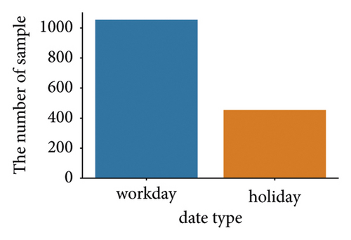
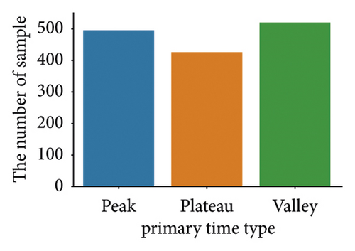
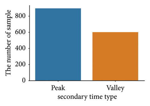
It is noted that all samples collected have four categorical features, namely, measurement time, date type, primary time type, and secondary time type. The measurement time represents the time information when the sample is measured, which ranges from 0 to 24 hours. The date type represents whether the measurement time is on a workday and holiday. The primary time type and secondary time type have two different definitions for daytime. The primary time type has three levels: peak mean hours refer to 09:00 to 12:00 and 18:00 to 21:00 daily, plateau mean hours refer to 13:00 to 17:00 and 22:00 to 23:00 daily, and valley represents 00:00 to 08:00. The secondary time type has two levels: peak means 08:00 to 21:00, whereas valley refers to 22:00 to 07:00. The distribution of these four categorical features is shown in Figure 8.

4. Results and Discussion

Before discussing the results, some hyperparameter settings of each method are described as follows. The prior weight and number of started jobs are set as 1 and 20 for TPE, and the rate of reduction in SA is 0.1 as default value. The learning rate is 5e − 4 in AGBO-based methods. The maximum of iteration step is 1000 for all the methods in this study. The parameter identification results of AGBO and SMBO-based methods with mean square error between U_c and U_cal are shown in Table 2.

It can be found in Table 2 that AGBO-Pro has the best performance with significantly low values of MAE, RMSE, and MAPE compared with other metaheuristic algorithms such as AO, NRO, and PSS. AGBO also has better results than SMBO-based methods, but the prediction results do not have remarkable differences since the statistical properties between U_c and U_cal are neglected.

Other recent studies also have proposed the prediction results with the same metrics and the same dataset in this paper, such as the methods of MCMC and SMBO combined with clustering and hypothesis testing (denoted as MCMC_C and SMBO_C). Li et al. [32] published the best results of MAE values of MCMC_C and SMBO_C being 62.467 ± 0.366 and 61.868 ± 0.322, respectively. In another paper [31], the values of MAE computed by MCMC_C and SMBO_C are 62.136 ± 0.336 and 61.268 ± 0.311, respectively.

Based on the previous study [26], the line transformation should be implemented to U_cal before calculating loss function. The parameter identification results with linear transformation are listed in Table 3.

All methods perform better in Table 3 than the results in Table 2, which indicates that the linear transformation between U_c and U_cal has an important contribution to identify PDN’s parameters. Moreover, the results between AGBO-Pro and AGBO mean that the supplementary categorical information such as measurement time, date type, primary time type, and secondary time type plays an important role in PDN’s parameter identification and the key categorical information can be merged by AGBO-Pro proposed in this work.

Leaning rate, the size of the embedding layer dimension, and the number of hidden layers are three critical hyperparameters of AGBO-Pro; therefore, the PDN’s parameter identification performance under different hyperparameters has been investigated in this section. The performances of various learning rates are displayed in Table 4.

It can be found that the learning rate has a remarkable influence on AGBO-Pro; when the learning rate is set to 5e − 3, the identification performance is optimal, and the value of learning rate between 1e − 2 and 1e − 3 is suggested in this paper. The size of embedding layer dimension is investigated subsequently under the optimal value of learning rate and listed in Table 5.

Since the dimension of categorical features is small, the embedding dimension of the neural network is less than 128 in this work. According to the results in Table 5, the change of the embedding dimension has only a minor impact on the identification performance, and the optimal size of the embedding dimension is chosen as 64, 32, 32, and 32 for the four categorical features, respectively. AGBO-Pro include the hidden layer to leaning the information of categorical features after embedding, and the influence of the number of the hidden layers are shown in Table 6.

Having more hidden layers in the network implies a larger number of parameters, slower computation speed, and a higher risk of overfitting. Combining the results from Table 6, it can be found that a single hidden layer achieves better identification performance. The convergence plots of AGBO and SMBO-based methods are displayed in Figure 9.

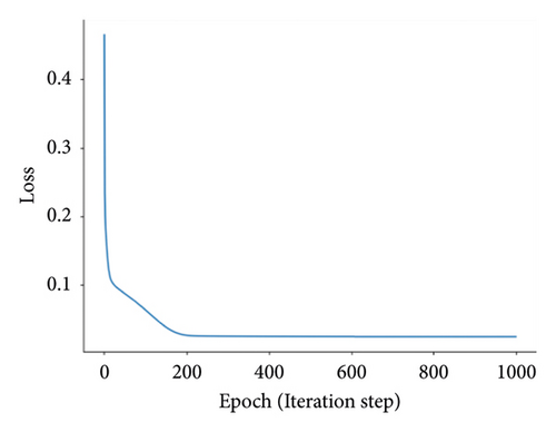
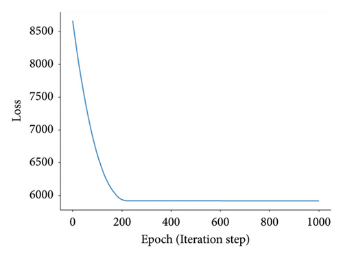
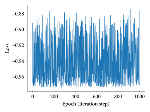
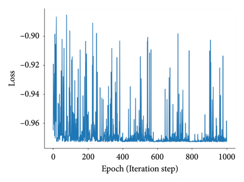
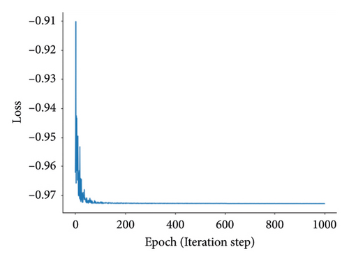
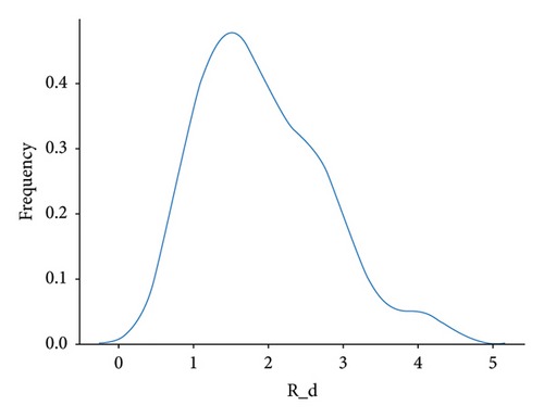
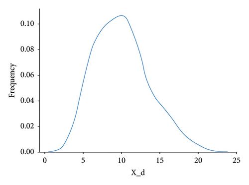
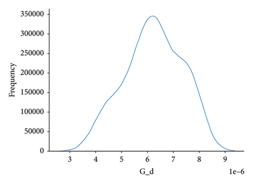
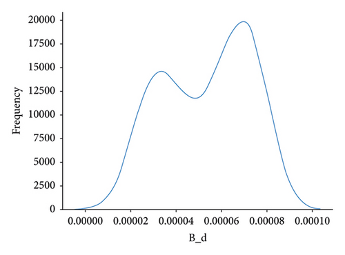
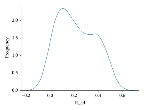
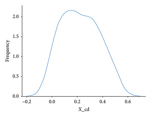
The AGBO-based methods converge after 200 iterations; compared with the SMBO-based methods, the convergence plots of AGBO-based methods are much smoother and stable, since the searching direction for parameter update is deterministic to the gradient-based optimization method, such as AGBO and AGBO-Pro. After 25 repeated splitting datasets, the distribution plots of the identified PDN’s parameters from AGBO-Pro-LR are shown in Figure 10. It can be found that all the identified parameters are roughly distributed within a relatively fixed range, providing a data foundation for the subsequent parameter analysis in future research.

5. Conclusion

In this work, we propose an extensible gradient-based optimization method for parameter identification in PDN calculation and analysis. A physical-informed multihead neural network is adopted to treat the numerical features and categorical features separately. The two kinds of features are merged via a weighted average. After several forward-backward calculations, the similarity loss function with respect to the six parameters to be identified achieves a fast convergence.

We compare the proposed method (namely, AGBO-Pro model) with the original AGBO model and several heuristic algorithms such as RS, TPE, SA, AO, NRO, and PSS. The numerical calculations show that the errors by AGBO-Pro are the lowest in all three evaluation functions, i.e., MAE, RMSE, and MAPE, with a faster and more stable convergence of the loss function. By further taking a linear transformation of the loss function, the method of this work has a lower variance in 25 repeat experiments, showing a much more robust performance in parameter identification.

In addition, the variations in hyperparameters of optimization method such as the number of hidden layers and embedding layers, learning rate, and weight decay are also systematically investigated. It is found that the method proposed in this work achieves more stable and robust performance to identify PDN parameters. This work shows an effective exploration in incorporating the numerical and categorical features of experimental measurement into gradient-based optimization method.

Conflicts of Interest

The authors declare that they have no conflicts of interest.