Aiming at the problems of incomplete classification features extraction of remote sensing images and low accuracy of crop classification in existing crop classification and recognition methods, a crop classification and recognition method using improved U-Net in Unmanned Aerial Vehicle (UAV) remote sensing images is proposed. First, the experimental data set is preprocessed. The data set is expanded by flipping transformation, translation transformation, and random cutting, which expands the number of data sets, and then the original image is cut to meet the requirements of the experiment for image size; Moreover, the network structure of U-Net is deepened, and the atrous spatial pyramid pooling (ASPP) structure is introduced after the encoder to better understand the semantic information and improve the ability of model mining data features; Finally, in order to prevent the overfitting of the deepened model, the dropout layer is introduced to weaken the joint adaptability between various neurons. Experiments show that the comprehensive OA and Kappa indexes of the proposed crop classification and recognition method based on improved U-Net are 92.14% and 0.896, respectively, which are better than the comparison methods. Therefore, the proposed method has good ability of crop classification and recognition.

1. Introduction

With the rapid development of industrialization and urbanization and the continuous improvement of China’s economic level, it provides a good environment for agricultural production but brings more challenges. The sustainable development and modernization of agriculture has gradually become the focus of relevant government departments [1, 2]. China is a large agricultural country. Crop cultivation is characterized by wide regions, great differences, and great seasonal changes. The main goal of agricultural production is to guide and adjust the macro planting situation from the national level to meet the needs of social development [3–6]. The traditional general survey of crop planting mainly adopts the agricultural statistical reports submitted from countryside to nation level upon level and adopts the catalog sampling method based on statistics. These methods are not only time-consuming and labor-consuming but also difficult to provide the geographical and spatial distribution information of crops, which cannot meet the requirements of today’s society for rapid mastery and management of agricultural production information [7–9], Therefore, it is of great strategic significance for food security to study how to accurately and efficiently obtain the type and scale of crop planting, analyze the information of crop planting structure, provide basic agricultural information source for government departments, and help them strengthen agricultural management and improve economic production [10].

Remote sensing technology is a technology that can sense the characteristic information of objects from a long distance to detect and recognize objects [11–13]. In recent years, remote sensing technology has become an effective technical means to identify crop types in a wide range [14, 15].

Among many crop classification algorithms, deep learning method is considered as a breakthrough technology and is increasingly applied to the field of crop recognition [16–18]. Deep learning network has a deeper and more complex structure, which can automatically learn the features inside the network layer, so as to achieve better crop recognition. In the process of crop classification and recognition, some crops are difficult to distinguish due to similar spectral features, salt and pepper noise, and low resolution of crop mapping, which seriously affect the accuracy of crop classification and recognition [19].

With the continuous progress of remote sensing technology, it is possible to carry out a wide range of crop classification research through remote sensing images [20]. Using conventional classification methods to extract remote sensing data is usually difficult to use the high-dimensional features covered by the image, and the classification effect is poor. Deep learning method can learn deeper features of images, extract them effectively, and make decision according to the target requirements. In recent years, the application scope of deep learning has been further expanded, which brings a new way to get better classification results of UAV remote sensing images. Reference [21] combined the advantages of deep spatial-temporal-spectral feature learning module and proposed a crop classification and recognition method based on recurrent neural network (RNN), which has better crop classification effect on time series multispectral images. Reference [22] inputted multitemporal remote sensing images into Conv1D network to classify crops based on pixels and obtained high classification accuracy. The existing image block-based classification methods often use three-dimensional convolution kernel to extract spatiotemporal features, which can effectively improve the phenomenon of salt and pepper noise. According to the structure of multispectral and multitemporal remote sensing data, reference [23] designed a three-dimensional CNN framework with fine-tuning parameters for training three-dimensional crop samples and learning spatiotemporal resolution representation and introduced an active learning strategy to improve the efficiency of the algorithm. Reference [24] used dual-channel convolutional neural network to extract temporal and spatial features from LiDAR data and then classified land cover types based on image blocks, so as to achieve high crop recognition accuracy on four data sets. Reference [25] used EVI series and time series feature representation network Conv1D for large-area crop classification based on pixels. Reference [26] used multitemporal Sentinel-2 data and GF-2 data as data sources. Sentinel-2 data were used as training data, and GF-2 data were used as verification data. A crop classification method based on convolutional neural network (CNN) and Visual Geometry Group (VGG) is proposed to classify crops. Reference [27] selected the target decomposition method to calculate the multidimensional feature images of the target and constructed a PolSAR classification model based on ResNet. However, when the above methods classify and recognize the remote sensing images of crops, there are often some problems, such as incomplete extraction of remote sensing image classification features and low classification accuracy.

2. Data Acquisition and Preprocessing

2.1. Overview of the Study Area

The study area is located in the crop planting area of Chifeng City, Inner Mongolia Autonomous Region, Northeast China, covering an area of about 500 square kilometers. The field survey was conducted from May to September 2020, which is the main growing season of crops. The crops in the study area are densely planted. In total, 127 experimental measurements were carried out on four land cover types of wheat, sunflower, corn, and soybean, as shown in Table 1.

1. Number of experimental measurements for each land cover type.

Serial number	1	2	3	4	Total
Type	Wheat	Sunflower	Corn	Soybean
Quantity	30	45	20	32	127

2.2. UAV Data Acquisition and Preprocessing

In order to obtain the high-resolution remote sensing image data of typical crops in the study area, the CW-10 composite wing UAV developed by Chengdu Zongheng Dapeng Company is selected as the flight platform, and the imaging devices are Sony RX0 visible light camera and Micasense five-channel multispectral camera. As shown in Figure 1, the composite wing UAV is equipped with remote sensing imaging equipment to obtain the high-resolution remote sensing image of crops.

Details are in the caption following the image — Open in figure viewer PowerPoint

As an industrial flight platform, the CW-10 composite wing UAV adopts conventional fixed wing combined with four rotor layout, with a wingspan of 2 m, a fuselage length of 1.3 m, an endurance of 60 min, a maximum takeoff weight of 6.8 kg, a payload of 800 g, a cruise speed of 65 kmh, a maximum flight speed of 100 km/h, and a wind resistance of level 6. It is used in conjunction with CW Commander and GCS-202 ground station. With the help of RTK/PPK positioning technology, the position information of remote sensing image can reach the centimeter level. In the experimental process, the designed flight altitude is 400 m, the speed is 20 m/s, the course overlap rate is 65%, and the side overlap rate is 70%. Route planning and task monitoring are carried out by using the supporting ground station software CW Commander. Remote sensing imaging equipment mainly include Sony RX0 visible light camera and Micasense multispectral camera. Sony RX0 has 24.00 mm main focal length, CCD size of 2.75 um, and effective phase amplitude of 13.2 × 8.8 mm, effectively preventing distortion through 1/32000 second high-speed electronic shutter. Micasense multispectral camera has five bands: blue, green, red, red edge, and near-infrared. The overall mass is 173 g, and the size is 9.34 cm × 6.3 cm×4.6 cm, also suitable for UAV flight load.

After two sorties, remote sensing images of typical crops were obtained, covering an area of more than 13000 mu. The spatial resolution of visible light data is 0.05 m, and the spatial resolution of multispectral data is 10 m, including a variety of ground feature information such as wheat, sunflower, corn, and soybean. After the mission, download the flight record data from the ground station, mobile station, and ground station software, respectively, and then import the record data to JoPPS solution software to obtain the location information of each shooting point of the corresponding aerial photography mission. The information includes the time, name, altitude, longitude and latitude, pitch angle, yaw angle, and other data records of the corresponding remote sensing data. The RTK/PPK positioning technology used during the flight, which can provide the three-dimensional positioning results of the survey site in the specified coordinate system in real time, and provide a good positioning basis for subsequent image stitching.

2.3. Data Set Production

The data set used in the study is mainly from UAV remote sensing images, which covers four labeled remote sensing images. The specifications of the four images are different, and the maximum value of the specification is 55128 × 49447. For this data set, it covers a variety of objects: wheat, sunflower, corn, and soybean, as well as other backgrounds.

In deep learning training, if the number of training samples is too small, there will be overfitting phenomenon, that is, the model overfits the data on the training set and reduces the prediction accuracy on the validation set. At present, the amount of training set data is small. Therefore, the sample data set on the experiment is trained through data expansion. The number of samples in data set is expanded by flipping, translating up, down, left, and right, and randomly cutting. After preprocessing, the data set is repartitioned, of which 80% is the training set and the remaining 20% is the validation set. Because the maximum image size is 55128 × 49447, which cannot be directly used for training. In order to meet the requirements of GPU storage and subsequent experiments on image size, the original image is cut into small pieces as the training set. The cutting method used in this paper is to slide on the original image for cutting. The size of the first cut image is 8000 × 8000, skipping the completely transparent part directly, and then cut the data set for the second time. The size of the second cut image is 1024 × 1024. In order to ensure the full coverage of data, the overlapping area is 128 × 128, cutting one block every other 128 pixels. Finally, 12168 images are obtained, of which 9735 are used as the training set, with a size of 1024 × 1024 × 8, and 2433 as verification sets, with a size of 1024 × 1024 × 8. The number of samples is greatly increased to meet the requirements of the experiment.

3. Crop Classification of Remote Sensing Images Based on Improved U-Net

3.1. U-Net Structure and Application

Due to the influence of its own structure, the traditional CNN network is difficult to classify images at the pixel level. In order to complete the recognition of a pixel, it is often necessary to input the pixel and its surrounding area into the network as a pixel block for prediction, resulting in large storage overhead and low calculation efficiency in the training process, and the perceived area is also limited by pixel blocks. As an improved convolutional neural network model, U-Net was proposed by Professor Oronneberger of Fitzburg University in 2015. Unlike other models used for scene image classification, U-Net was originally designed mainly for the features that are difficult to segment and extract in medical images, so as to try to recover the category of each pixel from the general features, that is, the classification is further extended from the image level to the pixel level. The overall composition of the model is shown in Figure 2. The most remarkable feature of U-Net network is to integrate low-dimensional features and high-latitude features and make full use of the semantic features of images. The structure of U-Net network is symmetrical.

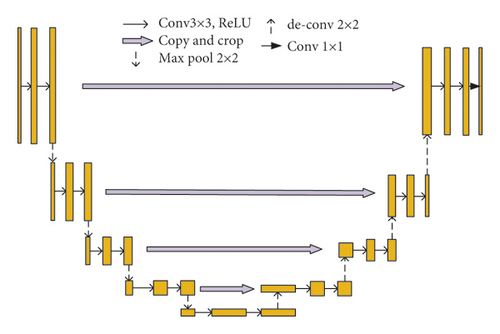
The main body of the U-Net model consists of 9 layers. In order to complete feature extraction and reconstruction, each layer of the network is composed of different numbers of convolution, pooling, deconvolution, and other operations. From a geometric point of view, the whole model presents a U-shape, which can be divided into two main bodies with the middle as the boundary, namely, feature extraction on the left and feature reconstruction on the right. The feature extraction process is similar to the typical convolution neural network process. The feature map is extracted in the way of convolution and pooling. At this stage, with the increase of network depth, the dimension of feature maps is also expanding. In contrast to the left channels, the right channels use deconvolution and concatenating to reduce the dimension of the extracted features. First, deconvolution is used to reduce the dimension of the feature maps, and then the corresponding part of the feature maps is concatenated to expand the size of the feature maps and repeat such operations until the last output layer.

3.2. Improved U-Net Model

3.2.1. Integration of U-Net and ASPP Module

ASPP module realizes the pyramidal dilated pooling in the spatial dimension. For ASPP module, it can provide good support for pyramid dilated pooling. This kind of design completes the sampling with a variety of dilated convolution for the preset input, which is equivalent to capturing the relevant data of the image through several scales. Using shortcut to stack the input and output generated by ASPP module will not significantly improve the amount of calculation of the network, but it can effectively increase the training efficiency of the model and optimize the actual training effect. In the process of deepening the model parameters, the ASPP structure can effectively deal with the degradation problem. The ASPP structure is shown in Figure 3, and the calculation formula is

\begin{matrix} Y = concat (I_{p} (X), H_{1,3} (X), H_{6,3} (X), H_{12,3} (X), H_{18,3} (X)), \end{matrix}

(1)

where concat() is feature map concatenating on the first dimension, H_i,j(X) represents the dilated convolution with kernel size of j, and sampling rate of i. I_p is all image-level features of the image pooling branch, which is an average pooling feature of the input feature map.

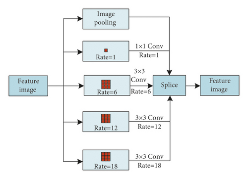
3.2.2. Classification Model Based on Improved U-Net

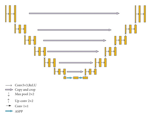
The overall architecture of the improved crop classification model is shown in Figure 4, which covers the basic structure of U-Net. In order to increase the training efficiency of the model, ASPP structure is added at the position where the lowest encoder and decoder connect with each other. Therefore, context semantic information can be generated under the condition of multiple sampling rates to better identify pixels, so as to ensure the most ideal classification effect. Two layers are added on the original U-Net structure, so the symmetrical structure of U-Net is expanded to a certain extent. Relatively more layers can form more semantic information, and the final features are more comprehensive. It ensures that there will be no gradient explosion after deepening and carries out standardized classification and recognition of crops in remote sensing images. First, input the image and use convolution to extract the downsampled features. Second, enrich the downsampled features through ASPP module to prevent gradient explosion in the deepened network. Finally, deconvolute on the right to obtain the result image.

3.2.3. Add Dropout Layer

Overfitting is a common problem in deep learning models. It is generally through the integration of multiple trained models, but the time consumption is too long, which is not conducive to long-term development and is not suitable for projects with high time requirements. Dropout layer temporarily eliminates the activity of some neurons by artificially setting a value, so as to achieve the purpose of network slimming. This value is between (0,1). The larger the value, the more neurons are inactivated. When the dropout layer is added to the neural network, the neurons in the hidden layer will be reduced. Figure 5 is a detailed demonstration of the dropout layer.

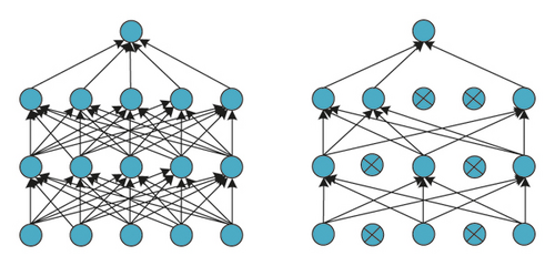
If the neuron is designated to be inactivated, the output data of the neuron are 0, and its weight value and bias value will not change, that is, during training, there are no inactivated nodes in the network, and these neurons cannot connected with other neurons. The model becomes simpler, and the amount of calculation is correspondingly reduced. Dropout layer will weaken the joint adaptability between various neurons and enhance the generalization ability.

3.2.4. Key Model Parameter Setting

The inputs of the proposed improved U-Net model are 5-channel remote sensing images, and the remote sensing data include red, green, blue, near-infrared, and NDVI band information. Set the pixel size of input data to 256 × 256. According to the observation, such size has sufficient context information, and the pixel category can be correctly judged even by visual interpretation. The number of images in the batch is increased by randomly applying flipping, rotation, and color jitter to the image block, so as to obtain sufficient sample data, avoid overfitting in the training process, and enhance the generalization ability of the model. The whole network structure is divided into 13 levels, and each level includes a different number of convolution, pooling, deconvolution, and other processes. In a typical convolution neural network structure, the number of feature maps is usually increased after the max-pooling operation to ensure the perfection of information. Considering that the upsampling operation has obtained relevant low-level features in the experimental training process, the downsampling operation is allowed to lose some information, and the experimental data are UAV remote sensing images, so there is no need to identify high-level 3D object concepts. The detailed parameter information of the model is shown in Table 2.

2. U-Net model parameters.

Process name	Processing parameters
Process name	Kernel size	Step	Edge padding	Post deconvolution padding
Cnov	3 × 3	1	1	—
Up-conv	3 × 3	2	1	1
Pool	2 × 2	1	0	—
Covn-out	1 × 1	1	0	—

The left side of the model is a compression channel, which is composed of convolution and pooling. The compression channel is used to extract image features layer by layer, reduce unnecessary weight connection, and reduce the impact of noise on the image. In order to avoid the problem that the training process converges more and more slowly with the deepening of the network, the model selects ReLu activation function. Whether in the forward or back propagation process, its convergence speed is better than Sigmod and Tanh function. At the same time, Batch Norm is added at some levels to ensure that the input of each layer of neural network maintains the same distribution through standardized means, so as to reduce the influence of gradient disappearance. The relationships between image input and output size in the compression process are expressed by equations (2) and (3):

\begin{matrix} y_{Cov} = \frac{x_{Cov} - k_{Cov} + 2 p + s_{Cov}}{s_{Cov}}, \end{matrix}

(2)

\begin{matrix} y_{pool} = \frac{x_{pool} - k_{pool} + s_{pool}}{s_{pool}}, \end{matrix}

(3)

where x_Cov is the input data of convolution operation, k_Cov is the convolution kernel size, p is the convolution padding size, s_Cov is the convolution step size, y_Cov is the output data of convolution operation, x_pool is the input part of the pooling operation, k_pool is the pooling kernel size, s_pool is the pooling step size, and y_pool is the output data of the pooling operation.

The size relationship between the input image and the output image is calculated by formula (2) every time after a convolution processing and by formula (3) every time after a pooling processing. The right side of the model is the extended channel, which mainly includes deconvolution, concatenating, and other processing processes. The concatenating process connects the feature maps of the corresponding level and changes the dimension of the feature maps without affecting the image size. As the inverse process of convolution operation, deconvolution gradually restores the feature maps to the original size by upsampling, which produces prediction for each pixel and retains the spatial information of the original image. The relationship between input and output size of image in the expansion process is as follows:

\begin{matrix} y_{up} = x_{up} s_{up} - s_{up} - 2 p_{up} + k_{up} + p_{op}, \end{matrix}

(4)

where x_up is the deconvolution input data, k_up is the deconvolution kernel size, s_up is the deconvolution step size, p_up is the edge padding size, and p_op is the padding size after deconvolution. The extended channel contains convolution part, but this process does not affect the image size. The last layer of the model is 1 × 1 × 1 convolution to obtain a single feature layer and use the Sigmoid function to map the pixel category of the feature map to the probability value between 0 and 1 to obtain the classification result. For the planting land to be classified, specific models are trained, respectively, according to the amount of data and data characteristics, so as to better fine-tune each type of network. In the training process, the batch size is set to 3, the learning rate is maintained at 0.001, and 100 epochs of training are carried out with the goal of minimizing the cross-entropy loss function.

4. Experiment and Analysis

4.1. Experimental Setup and Evaluation Index

This paper deepens the layers of U-Net network, which has certain requirements for computer during training, otherwise it takes a lot of time and affects parameter adjustment. The computer for training is Inter(R) Core(TM) i7-7700HQ CPU @2.80 GHz processor, TensorFlow2.0.0 GPU version; the computer for testing is Inter(R) Core(TM) i5-8250U CPU @1.60 GHz processor, TensorFlow2.0.0 CPU version. The software also has Python 3.6, Keras2.2.4.

The overall classification accuracy (OA), Kappa coefficient, precision (PR), recall (RC), F1 score, and intersection-over-union (IOU) are used as evaluation indexes. Overall classification accuracy (OA) refers to the ratio of the number of correctly classified crop pixels to the total number of crop pixels. Its calculation formula is

\begin{matrix} OA = \frac{\sum_{i = 1}^{n} p_{i, i}}{\sum_{j = 1}^{n} \sum_{i = 1}^{n} p_{i, j}}, \end{matrix}

(5)

where p_i,j represents the total number of pixels belonging to category i and assigned as category j and n represents the number of categories.

Kappa coefficient is calculated according to the confusion matrix, and its calculation formula is as follows:

\begin{matrix} Kappa = \frac{N^{2} \times OA - \sum_{i = 1}^{n} a_{i} b_{i}}{N^{2} - \sum_{i = 1}^{n} a_{i} b_{i}}, \end{matrix}

(6)

where N represents the total number of samples, a_i is the actual number of samples of each type, and b_i is the number of samples predicted by each type.

The precision represents the proportion of the number of pixels in the correct change area predicted in the prediction map to the number of pixels in all the real reference change areas. The recall represents the proportion of the change area correctly recognized by the algorithm in the change area of the original image. F1 score is related to both precision and recall, which is the reconciliation of precision and recall. IoU is to calculate the proportion between the intersection and union of two sets. In the remote sensing image change detection task, these two sets represent the changed area and the unchanged area. The calculation methods of the four indicators are shown in formulas (7) to (10).

\begin{matrix} Precision = \frac{TP}{TP + FP}, \end{matrix}

(7)

\begin{matrix} Recall = \frac{TP}{TP + FN}, \end{matrix}

(8)

\begin{matrix} F 1 = \frac{2 \times Precision \times Recall}{Precision + Recall}, \end{matrix}

(9)

\begin{matrix} IoU = \sum_{i = 0}^{k} \frac{p_{i i}}{\sum_{j = 0}^{k} p_{i j} + \sum_{j = 0}^{k} p_{j i} - p_{i i}}, \end{matrix}

(10)

where k represents the number of object categories; p_ij represents the number of pixels that belong to the category i but are recognized as the category j; p_ii indicates the correct number of identified pixels; TP represents the pixel marked as the change region in the reference image, and the recognition result of the algorithm for this region is also the pixel of the change region; FP represents the pixel marked as unchanged area in the reference image, and the recognition result of the algorithm for this area is the changed area; FN represents the region marked as changed in the reference image, and the recognition result of the region by the algorithm is the unchanged region; and TN represents the area marked as unchanged in the reference image, and the recognition result of the algorithm for this area is also unchanged.

4.2. Changes of Accuracy and Loss Value during Improved U-Net Training

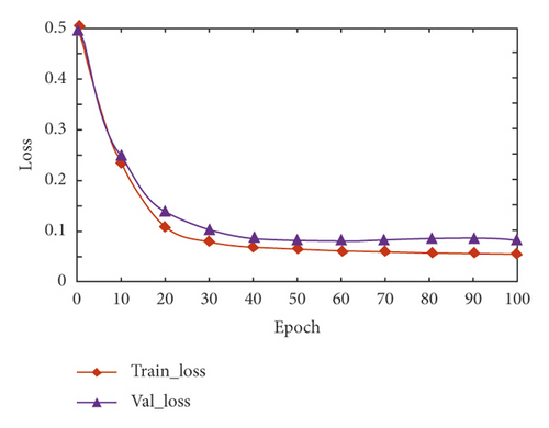
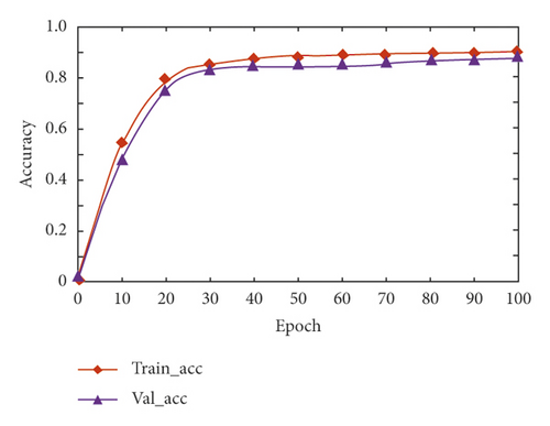
Three training samples are input into the training set at a time, and the parameters are updated iteratively through the cross-entropy loss function and Adam optimizer. Under the framework of Keras based on Tensorflow, using GPU acceleration, all training samples pass through 100 epochs to complete the model training of the proposed improved U-Net. Figure 6 shows the change curve of accuracy and loss value of training data and validation data in the training process of the network model. It can be seen that with the continuous increase of training iterations, the accuracy and loss value gradually remain stable. The improved U-Net model in this paper gradually tends to converge. When the epoch is 20, the loss value and accuracy are stable, Train_loss and Val_loss have converged and the difference between them is very small. Finally, Train_loss is stable at about 0.05, Val_loss is stable at about 0.11, Train_acc is stable around 0.88, and Val_acc was stable at 0.83. Dropout layer is introduced into the proposed model, which weakens the joint adaptability between various neurons, enhances the generalization ability, and effectively prevents the overfitting problem of the depth model.

4.3. Comparison of Accuracy of Extraction Results between U-Net and Improved U-Net

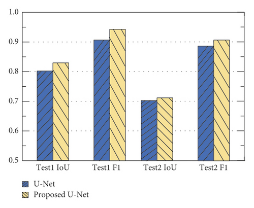
In order to objectively analyze the crop classification results of the proposed improved U-Net model, two evaluation indexes IoU and F1 score are used to quantitatively compare the accuracy with the original U-Net extraction results based on the corresponding truth label. The comparison results are shown in Figure 7. It can be seen from Figure 7 that the extraction accuracy of the proposed improved U-Net model is not significantly improved compared with the original U-Net in test area 2. However, in test area 1, compared with the results before the improvement, the extraction accuracy of the improved U-Net model is improved by about 4%, and the IoU and F1 score values reach 0.8358 and 0.9397, respectively, which proves the effectiveness of the proposed improved U-Net model in improving the accuracy of crop classification and recognition.

4.4. Performance Comparison with Other Methods

In order to prove the advantages of the proposed crop classification and recognition method based on improved U-Net, classification methods in Ref. [26, 27] are compared with the proposed method under the same experimental conditions. The experimental results are shown in Table 3.

3. Comparison of different deep learning methods.

Method	Type	PR	Re	F1	IoU	OA	Kappa
Ref. [26]	Wheat	0.976	0.954	0.965	0.915	91.37%	0.874
	Sunflower	0.924	0.901	0.912	0.904
	Corn	0.953	0.914	0.933	0.901
	Soybean	0.629	0.817	0.711	0.610
Ref. [27]	Wheat	0.945	0.931	0.938	0.907	90.65%	0.864
	Sunflower	0.913	0.887	0.900	0.897
	Corn	0.927	0.904	0.915	0.878
	Soybean	0.614	0.811	0.699	0.601
Proposed method	Wheat	0.996	0.977	0.986	0.976	92.14%	0.896
	Sunflower	0.936	0.916	0.926	0.917
	Corn	0.983	0.924	0.953	0.926
	Soybean	0.685	0.845	0.757	0.641

Table 3 shows the comparative analysis of various crops by various deep learning networks on various evaluation indexes. The OA of Ref. [27] method is only 90.65%, and the Kappa index is 0.864. The OA of Ref. [26] method is 91.37%, and the Kappa index is 0.874. The OA of the proposed method is 92.14%, and the Kappa index is 0.896. These two indexes are the best. The accuracy of the proposed method in wheat, sunflower, corn, and soybean recognition is higher than that of the comparative method. For wheat, the four indexes of PR, Re, F1, and IoU of the proposed method are 0.996, 0.977, 0.986, and 0.976, respectively. For the soybean, the least number of samples, the four indexes of PR, Re, F1, and IoU of the proposed method are 0.685, 0.845, 0.757, and 0.641, respectively, which are better than the comparative methods. The proposed improved U-Net recognition and classification method adds ASPP structure at the junction of encoder and decoder (the lowest level of U-Net structure), which enhances the feature recognition ability of the method. It not only uses the feature information of wheat on the image but also combines the surrounding pixels for recognition and classification, so its accuracy and reliability are higher. The comparison method adopts multiple kinds of data sets, pursues the generalization performance of the model, but ignores the deep feature extraction of remote sensing image. Therefore, when dealing with the task of crop classification and recognition of remote sensing image, the values of each index are lower than those of the proposed method.

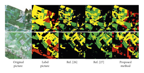
Figure 8 is a comparison diagram of some crop classification and recognition results between the proposed method and other algorithms. It can be seen from the classification results that the planting area of wheat is very concentrated and there are many samples collected, so the classification accuracy shown in the four models is very high. Therefore, it can be seen that the number and distribution of samples in different categories are also important factors that may affect the accuracy of crop classification. This is because the proposed method introduces ASPP structure and deepens the U-Net structure, which makes the proposed model better generate semantic information and improve the ability of mining data features. The two models of Ref. [26, 27] cannot fully and effectively integrate the feature information of crop remote sensing images, so the classification effect on the result map is poor. Therefore, experiments show that the proposed method is feasible and efficient for crop classification and recognition in UAV remote sensing images.

5. Conclusion

Aiming at the problems of incomplete extraction of classification features of remote sensing images and low accuracy of crop classification in existing crop classification and recognition methods, a crop classification and recognition method using improved U-Net in UAV remote sensing images is proposed. Aiming at the problems of traditional U-Net network, ASPP module is introduced to improve the accuracy of U-Net model in feature extraction, which is conducive to better terrain semantic information and obtain more comprehensive data features. Experiments show that the proposed method has good ability of crop classification and recognition.

In the follow-up, the high spatial resolution and hyperspectral resolution remote sensing images can be combined at the same time, using different methods to fuse, and analyze its impact on the classification effect. Moreover, the structure design and super parameter selection of deep learning network play a vital role in the learning ability of the network. The further research and improvement of deep learning model is also the focus of future research.

Conflicts of Interest

The authors declare that there are no conflicts of interest regarding the publication of this paper.

Acknowledgments

This work was supported by Inner Mongolia Science and Technology Plan Project “Diagnosis System of Sunflower Leaf Diseases Based on Image Recognition” (No. 61561038), and Inner Mongolia Electronic Information Vocational Technical College’s 2021-Year In-School Scientific Research “Research on Data Collection, Processing and Transmission of Smart Agricultural Environmental Monitoring Nodes” (No. KZY2021008).

Open Research

Data Availability

The data used to support the findings of this study are included within the article.

References

1 Orynbaikyzy A., Gessner U., and Conrad C., Crop type classification using a combination of optical and radar remote sensing data: A review, International Journal of Remote Sensing. (2019) 40, no. 17, 6553–6595, https://doi.org/10.1080/01431161.2019.1569791, 2-s2.0-85060925176.
10.1080/01431161.2019.1569791
Web of Science® Google Scholar
2 Wang A., Zhang W., and Wei X., A review on weed detection using ground-based machine vision and image processing techniques, Computers and Electronics in Agriculture. (2019) 158, no. 8, 226–240, https://doi.org/10.1016/j.compag.2019.02.005, 2-s2.0-85061429740.
10.1016/j.compag.2019.02.005
Web of Science® Google Scholar
3 Ennouri K, Smaoui S, Gharbi Y, Cheffi M, Braiek O. B, Ennouri M, and Triki M. A, Usage of artificial intelligence and remote sensing as efficient devices to increase agricultural system yields, Journal of Food Quality. (2021) 5, no. 2, 211–220, https://doi.org/10.1155/2021/6242288.
10.1155/2021/6242288
Google Scholar
4 Velesaca H. O, Suárez P. L, Mira R, and Sappa A. D, Computer vision based food grain classification: A comprehensive survey, Computers and Electronics in Agriculture. (2021) 187, no. 1, 106–116, https://doi.org/10.1016/j.compag.2021.106287.
10.1016/j.compag.2021.106287
Web of Science® Google Scholar
5 Liu C.-a., Chen Z.-x., Shao Y., Chen J.-s., Hasi T., and Pan H.-z., Research advances of SAR remote sensing for agriculture applications: A review, Journal of integrative agriculture. (2019) 18, no. 3, 506–525, https://doi.org/10.1016/s2095-3119(18)62016-7, 2-s2.0-85062423821.
10.1016/S2095-3119(18)62016-7
Web of Science® Google Scholar
6 Potgieter A. B, Zhao Y, Zarco-Tejada P. J, Chenu K, Zhang Y, Porker K, Biddulph B, Dang Y. P, Neale T, Roosta F, and Chapman S, Evolution and application of digital technologies to predict crop type and crop phenology in agriculture, In Silico Plants. (2021) 8, no. 1, 2674–2683, https://doi.org/10.1093/insilicoplants/diab017.
10.1093/insilicoplants/diab017
Google Scholar
7 Ray S. S, Singh R. P, and Choudhary K, Contribution of IRS-1C data to agricultural monitoring: A review, Journal of the Indian Society of Remote Sensing. (2021) 4, no. 2, 28–35, https://doi.org/10.1007/s12524-020-01282-6.
10.1007/s12524-020-01282-6
Google Scholar
8 Liakos K., Busato P., Moshou D., Pearson S., and Bochtis D., Machine learning in agriculture: A review, Sensors. (2018) 18, no. 8, 2674–2685, https://doi.org/10.3390/s18082674, 2-s2.0-85052088926.
10.3390/s18082674
Web of Science® Google Scholar
9 Srivastava P, Shukla A, and Bansal A., A comprehensive review on soil classification using deep learning and computer -ision techniques, Multimedia Tools and Applications. (2021) 3, no. 1, 1–28.
Google Scholar
10 Khan M. A., Akram T., Sharif M., Awais M., Javed K., Ali H., and Saba T., CCDF: Automatic system for segmentation and recognition of fruit crops diseases based on correlation coefficient and deep CNN features, Computers and Electronics in Agriculture. (2018) 155, no. 5, 220–236, https://doi.org/10.1016/j.compag.2018.10.013, 2-s2.0-85055152402.
10.1016/j.compag.2018.10.013
Web of Science® Google Scholar
11 Kaur S., Pandey S., and Goel S., Plants disease identification and classification through leaf images: a survey, Archives of Computational Methods in Engineering. (2019) 26, no. 2, 507–530, https://doi.org/10.1007/s11831-018-9255-6, 2-s2.0-85040678897.
10.1007/s11831-018-9255-6
Web of Science® Google Scholar
12 Koirala A., Walsh K. B., Wang Z., and McCarthy C., Deep learning - method overview and review of use for fruit detection and yield estimation, Computers and Electronics in Agriculture. (2019) 162, no. 4, 219–234, https://doi.org/10.1016/j.compag.2019.04.017, 2-s2.0-85064313579.
10.1016/j.compag.2019.04.017
Web of Science® Google Scholar
13 Mavridou E, Vrochidou E, Papakostas G. A, Pachidis T, and Kaburlasos V. G, Machine vision systems in precision agriculture for crop farming, Journal of Imaging. (2019) 5, no. 12, 82–89, https://doi.org/10.3390/jimaging5120089.
10.3390/jimaging5120089
PubMed Web of Science® Google Scholar
14 Iqbal Z., Khan M. A., Sharif M., Shah J. H., ur Rehman M. H., and Javed K., An automated detection and classification of citrus plant diseases using image processing techniques: A review, Computers and Electronics in Agriculture. (2018) 153, no. 2, 12–32, https://doi.org/10.1016/j.compag.2018.07.032, 2-s2.0-85050968013.
10.1016/j.compag.2018.07.032
Web of Science® Google Scholar
15 Lu B., Dao P., Liu J., He Y., and Shang J., Recent advances of hyperspectral imaging technology and applications in agriculture, Remote Sensing. (2020) 12, no. 16, 2659–2667, https://doi.org/10.3390/rs12162659.
10.3390/rs12162659
Web of Science® Google Scholar
16 Guo Q, Jin S, Li M et al., Application of deep learning in ecological resource research: Theories, methods, and challenges, Science China Earth Sciences. (2020) 5, no. 6, 1–18, https://doi.org/10.1007/s11430-019-9584-9.
10.1007/s11430-019-9584-9
Google Scholar
17 Zhang Q., Liu Y., Gong C., Chen Y., and Yu H., Applications of deep learning for dense scenes analysis in agriculture: A review, Sensors. (2020) 20, no. 5, 1520–1526, https://doi.org/10.3390/s20051520.
10.3390/s20051520
Web of Science® Google Scholar
18 Sheykhmousa M, Mahdianpari M, Ghanbari H, Mohammadimanesh F, Ghamisi P, and Homayouni S, Support vector machine vs. random forest for remote sensing image classification: a meta-analysis and systematic review, Ieee Journal of Selected Topics in Applied Earth Observations and Remote Sensing. (2020) 7, no. 1, 12–20.
Google Scholar
19 Kamilaris A. and Prenafeta-Boldú F. X., Deep learning in agriculture: A survey, Computers and Electronics in Agriculture. (2018) 147, no. 7, 70–90, https://doi.org/10.1016/j.compag.2018.02.016, 2-s2.0-85042262881.
10.1016/j.compag.2018.02.016
Web of Science® Google Scholar
20 Kamilaris A. and Prenafeta-Boldú F. X., A review of the use of convolutional neural networks in agriculture, The Journal of Agricultural Science. (2018) 156, no. 3, 312–322, https://doi.org/10.1017/s0021859618000436, 2-s2.0-85048966412.
10.1017/S0021859618000436
Web of Science® Google Scholar
21 Luo C, Meng S, Hu X, Wang X, and Zhong Y, Cropnet: deep spatial-temporal-spectral feature learning network for crop classification from time-series multi-spectral images, IGARSS 2020-2020 IEEE International Geoscience and Remote Sensing Symposium, 26 Sept.-2 Oct. 2020, Waikoloa, HI, USA, IEEE, 4187–4190, https://doi.org/10.1109/igarss39084.2020.9324097.
10.1109/igarss39084.2020.9324097
Google Scholar
22 Guidici D. and Clark M., One-Dimensional convolutional neural network land-cover classification of multi-seasonal hyperspectral imagery in the San Francisco Bay Area, California, Remote Sensing. (2017) 9, no. 6, 629–637, https://doi.org/10.3390/rs9060629, 2-s2.0-85021141369.
10.3390/rs9060629
Web of Science® Google Scholar
23 Ji S, Zhang C, Xu A, Shi Y, and Duan Y, 3D convolutional neural networks for crop classification with multi-temporal remote sensing images, Remote Sensing. (2018) 10, no. 1, 75–86, https://doi.org/10.3390/rs10010075, 2-s2.0-85040655409.
10.3390/rs10010075
Web of Science® Google Scholar
24 Xu X, Li W, Ran Q, Du Q, Gao L, and Zhang B, Multisource remote sensing data classification based on convolutional neural network, IEEE Transactions on Geoscience and Remote Sensing. (2017) 56, no. 2, 937–949.
10.1109/TGRS.2017.2756851
Web of Science® Google Scholar
25 Zhong L., Hu L., and Zhou H., Deep learning based multi-temporal crop classification, Remote Sensing of Environment. (2019) 221, no. 3, 430–443, https://doi.org/10.1016/j.rse.2018.11.032, 2-s2.0-85057535465.
10.1016/j.rse.2018.11.032
Web of Science® Google Scholar
26 Yang S, Gu L, Ren R, and He F, Research on crop classification in Northeast China based on deep learning for Sentinel-2 data, Earth Observing Systems XXIV, 2019, San Diego, CA, USA, International Society for Optics and Photonics, 111–119, https://doi.org/10.1117/12.2527376.
10.1117/12.2527376
Google Scholar
27 Mei X, Nie W, Liu J, and Huang K, Polsar image crop classification based on deep residual learning network, 2018 7th International Conference on Agro-geoinformatics, 6-9 Aug, 2018, Hangzhou, China, IEEE, 1–6, https://doi.org/10.1109/agro-geoinformatics.2018.8476061, 2-s2.0-85055896422.
10.1109/agro-geoinformatics.2018.8476061
Google Scholar

Citing Literature

All articles

Intelligent Identification Method of Crop Species Using Improved U-Net Network in UAV Remote Sensing Image

Abstract

1. Introduction