Literature is extremely important in the advancement of human civilization. Every day, many literary texts of various genres are produced, dating back to ancient times. An urgent concern for managers in the current literary activity is how to classify and save the expanding mass of literary text data for easy access by readers. In the realm of text classification, the TF-IDF algorithm is a widely used classification algorithm. However, there are significant issues with utilizing this approach, including a lack of distribution information inside categories, a lack of distribution information between categories, and an inability to adjust to skewed datasets. It is possible to improve classification accuracy by using the TF-IDF algorithm in this paper’s application situation by exploiting the association between feature words and the quantity of texts in which they appear, while ignoring the variation in feature word distribution across categories. With the purpose of classifying the literary texts in this study, this work proposes an improved IDF method for the problem of feature words appearing several times and having diverse meanings in different fields. The meanings of feature words in distinct domains are separated to increase the trust in the TF-IDF algorithm’s output. Using the improved TF-IDF method suggested in this research with the random forest (RF) classifier, the experimental results show that the classifier has a good classification impact, which can meet the actual work needs, based on comparative experiments on feature dimension selection, feature selection algorithm, feature weight algorithm, and classifier. It has a fair amount of historical significance.

1. Introduction

As the world entered the twenty-first century, it saw rapid development, with all kinds of new things sprouting up like mushrooms after a rain and people’s lives and society taking on a new look. While new things are constantly emerging, some excellent traditional cultures are in danger of extinction. Under these conditions, preserving and promoting excellent traditional culture have become a hot topic. Literature is the core connotation of excellent traditional culture because it is a record and inheritance of traditional culture. The soil and conditions for the spread of excellent traditional culture are provided by literature. As time passes, more and more excellent literary works are created, and the preservation and retrieval of digitized literary texts face new challenges. Text classification technology is essential in such a massive data base for quickly and accurately obtaining the required information from the massive and disorganized literary texts. Text classification used to be done by hand. Manual information extraction could not meet people’s needs in the face of the exponential growth of text information. This must assist users in obtaining valuable information quickly and accurately by utilizing computers’ ability to process information automatically, quickly, and in large quantities.

American scientist Dr. Luhn proposed a system for automatically writing article abstracts in the 1950s. This method counts the frequency of words and sentences in the paper or article and their spatial distribution information [1]. Thus, for the first time, abstract writing is automated. This technical method shows a rapid progress in text classification [2]. In July, Maron and Kuhn published their first text classification paper in the ACM magazine, describing a new method for bibliographic indexing and searching in libraries [3]. Although these methods are still in the experimental stage, they may pave the way for future statistical text classification technology. Text classification now uses machine learning [4, 5] and deep learning [6, 7] techniques. KNN and Naive Bayes are commonly used methods in machine learning [8]. In text classification, Joachims employed support vector machines [9], and ensemble learning approaches worked well in text classification, Chen et al. proposed a scalable end-to-end model XGBoost based on boosting [10]. The Microsoft AI Research Institute proposed the LightGBM boosting model [11] which is faster and uses less memory than XGBoost training. In 2017, the Russian search company Yandex released the “super-combat” machine learning model CatBoost [12]. In recent years, the integrated learning model represented by XGBoost, LightGBM, CatBoost, and so forth has swept the major data mining contests, demonstrating the rapid progress of machine learning. Obtaining tagged text data is typically time-consuming and difficult. Reference [13] usesd the available labeled documents to train the classifier, then randomly labeled the unknown documents with a certain probability, and iterated until convergence. Deep learning employs text as a word vector to classify [14]. Yoon extracted text features and performed well in text categorization [15]. Multilayer convolution and pooling layers learn more detailed semantic information. RNNs are naturally better at processing text-like serialized data. RNNs can parse extended sequences and capture textual context dependencies. As a result, RNNs have obvious gradient dispersion and gradient explosion issues during training [16]. Later, Schmidhuber suggested an updated model of RNN, LSTM [17], with memory, forget, and output gate units to overcome the gradient dispersion problem in backpropagation. The LSTM model is used for text classification with impressive results. Zhou et al. [18] proposed a C-LSTM model that combines convolutional and recurrent neural networks’ benefits. The design is straightforward and end-to-end by combining n-gram features with a single-layer CNN. A higher-level representation of in-text sequential relationships is learned by deriving a single structure from the input sentence.

The comparative analysis of the above studies reveals that the machine learning algorithm’s text classification and recognition speed is fast, and the model training is relatively simple, but the recognition rate is not as high as that based on the deep learning algorithm. However, the deep-learning-based text classification model has many training parameters, takes a long time, and requires powerful hardware. If the recognition rate of machine-learning-based text classification can be improved further, the time-consuming issues caused by deep learning algorithms can be avoided. This study proposes an improved TF-IDF method combined with an RF classification algorithm to classify literary texts based on this. Results from an experiment show that the methods proposed in this paper can achieve the desired results and have commercial value. The main contribution of this paper is as follows: First, it is situated in the field of literary text classification, which is currently understudied. Second, this paper proposes and theoretically validates an improved TF-IDF method for text classification tasks. Third, the superiority of the text classification method used in this paper is demonstrated by experimental comparison using self-created experimental data.

2. Relevant Knowledge

2.1. Definition of Text Classification

Text classification technology specifically refers to the establishment or selection of appropriate classification rules for the text data to be classified according to the characteristics of its text content in some aspects (mainly different viewpoints or topics appearing in the text). The basic process of establishing the classification rules is as follows: Firstly, the classification rules are searched backward from the classification results, that is, according to the different characteristics of different types of texts from the classified training texts, and then certain accurate and appropriate classification rules are searched and extracted. Then the text is classified according to the above rules, and finally the classification result is made consistent with the target result, thus obtaining a good text classification model.

When it comes to the foundations of text classification, the set mapping connection serves as a good analogy. The goal of text classification is to summarize and extract appropriate classification rules from the classified texts in order to classify the remaining unclassified texts correctly. To obtain the correct classification result, it must use an algorithm to determine the degree of association between the text object and each category based on the distribution and characteristics of the text objects and then select the appropriate classification threshold based on the relationship of the degree of association. Equation (1) shows the text categorization calculation formula and can be defined as follows:

(1)

where T represents true and F represents false. The set X = {x₁, x₂, …, x_i, …, x_n} in equation (1) refers to the set of texts to be classified, where x_i represents the i-th text to be classified and n refers to the text to be classified. The number of texts to be classified is contained in the classification text set X. Set C = {c₁, c₂, …, c_j, …, c_h} denotes our predefined category set, where c_j denotes the jth category and h denotes the number of predefined categories in category set C. A mapping relationship is represented by the S function. For example, if S(x_i, c_j) = T, the classification result of the i-th text to be classified x_i in the dataset is the j-th category c_j. Otherwise, if S(x_i, c_j) = F, the classification result of the i-th text to be classified x_i in the dataset is not the j-th category. Because mathematical collections have two mapping relationships of one-to-one and one-to-many mapping concepts, text classification can also be divided into single-label classification and multilabel classification. Label-only classification is one of them. Only one category can be assigned to the text to be classified. At this point, two scenarios are possible: binary classification and multiclassification. A typical binary classification application is spam classification. Because news websites have many columns, their news classification systems are frequently multiclassification applications, with multilabel classification referring to the possibility of classified texts being classified into two categories at the same time.

2.2. Text Classification Process

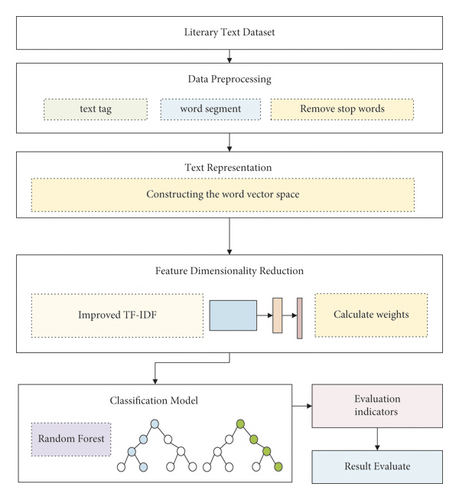
Text data preparation, text representation, feature dimension reduction, classification model training, classification performance evaluation, and other procedures are all common processing links in today’s widely recognized text classification approaches. Figure 1 depicts the basic text classification method.

Details are in the caption following the image — Open in figure viewer PowerPoint

The initial processing step after receiving the dataset is to do data preprocessing on the text data in order to achieve the goal of automatic text categorization. We must do the following operations on the text data in this procedure, according to the processing order: text tagging, word segmentation, and stop word removal.

Following the text preprocessing link, the text data obtained at this time is most likely as follows: “She/love/sports.” These are all character data and do not present the text’s structured information. Even if this data is entered into a computer, the computer will not be able to directly use and perform subsequent text classification. As a result, further processing of the text data is required at this time. In general, the text is represented as a formal or mathematical description by a specific method, so that it can be recognized by a computer. This is the function that should be implemented in the text representation link, and the text data processed by this link can aid in subsequent classification. In general, words form sentences, sentences form paragraphs, and paragraphs form documents; thus, words are the finest granularity among them, and the text representation process can be divided into different granularities, which can realize text word division. There are several methods for dividing phrases, sentences, and paragraphs. The text representation is a translation of the text in Chinese into a binary language that the computer can recognize and process. Domestic text representation models currently include the Boolean model, the VSM model, and the statistical language model.

Dimensionality reduction is a fundamental concept in data statistics. The goal of feature dimensionality reduction in this case is to completely preserve the original text features via data dimensionality reduction. Not only does feature dimensionality reduction reduce the amount of classification calculation, but also it plays an important role in improving classification accuracy and efficiency, as well as avoiding the phenomenon of classifier overfitting. For text data, feature selection is a common feature dimensionality reduction method. The general processing flow of feature selection is as follows: based on the characteristics of the text dataset, select a suitable feature calculation function through the selection process and perform feature calculation on each term in each text in the dataset to obtain quantified results, with the results sorted from largest to smallest. Arrange from from big to small, select a certain number of feature items as the representative of the original text data based on a predetermined threshold, and do not involve feature space transformation during this period.

The dataset can be categorized after it has been reduced in dimensionality by features. Most often used text classification methods include the Naive Bayes algorithm, K-nearest neighbor algorithm, decision tree algorithm, support vector machine, convolutional neural network, recurrent neural network, and others. Naive Bayes algorithm is one of the most widely used algorithms.

3. Application of Improved TF-IDF Method in Literary Text Classification

3.1. Traditional TF-IDF Algorithm

For the TF-IDF algorithm, the feature word is assigned a weight based on how frequently it appears in the document set. If one category has many documents with the same feature word, the feature word has a good capacity to represent it. The feature word, strong, should be given more weight. However, if the feature word is common across all categories, regardless of how many times it appears in each document set, it should be given a lower weight.

In order to get the weight of the feature word, the word frequency is multiplied by the inverse document frequency. It is the frequency of the feature word in the document inside the class, and the inverse document frequency is the distribution information for the feature word occurring in many categories. There are two pieces to the TF-IDF algorithm’s formula: TF and IDF. The frequency of words in a class is represented by the term “word frequency,” abbreviated as “TF.” IDF is an abbreviation for the cross entropy of feature word probability density. The traditional algorithm’s calculation is shown in the following equation:

(2)

where H_i is the weight result obtained by the feature word, C_i is the number of occurrences of the feature in the document, T is the total number of files, t_i is the number of documents in which the feature word has appeared, and γ is an empirical value, typically 0.01.

Equation (3) is used for normalization processing:

(3)

When it comes to document length, the longer the document is, the more characteristic words it will contain. Words that appear repeatedly in the document will be given higher weights, even if they are not very useful for classification. Similarly, when a document is short, it has fewer feature words and each word appears less frequently than words in other documents. Its classification ability for these words may be very strong, but it is obtained with a lower weight. The normalized form has the advantage that the calculation formula provides a “fairer” measure of the TF value regardless of document length. The TF-IDF algorithm’s calculation formula reveals that the algorithm calculates the weight of the feature word using two variables: the feature word’s word frequency and the inverse document frequency of the feature word. As a result, using the algorithm formula to calculate the weight of the feature word can better reflect the occurrence information of the feature word in the document set and partially reflect the distribution information of the feature word among the categories. However, when classifying the model using the above algorithm’s actual training, the classification accuracy remains low, and the algorithm can still be continuously improved.

The formula reveals that T represents the sum of the numbers of documents, implying that T does not contain information about the distribution of feature words across multiple categories. According to the algorithm’s principle, when feature words appear frequently in most categories, they should be given a lower weight. However, the weight calculation is also influenced by the feature words’ frequency. The calculated weight value is frequently determined by the feature words’ frequency. The weight value may be excessive. When the number of occurrences of feature words in this document remains constant while the frequency of occurrence of other documents in this category increases, the IDF should increase accordingly. However, the IDF part of the formula does not consider the frequency of occurrence of feature words in this category and only focuses on occurrences or not, so the IDF calculation result does not change. Furthermore, when the number of documents varies greatly across the dataset’s categories, the IDF value calculated by the category with the fewest documents has little classification effect. It is impossible to adjust the IDF value when the frequency of feature words in a category remains constant, since feature word distribution is not taken into consideration by IDF. Feature word distribution in a document collection is not accurately represented by the IDF section of the calculation because of the random distribution of feature words in the class.

3.2. TF-IDF Algorithm Defects

Based on an investigation of the standard TF-IDF method, the following shortcomings are summarized:

(1)
No distribution information within the category. Because the document collection is organized hierarchically, it usually takes the form of a two-level directory. That is, the first level is a collection of documents distinguished by categories, while the second level is a collection of documents within the same category. If you are only using the TF-IDF technique within one category, you will only be calculating occurrences of feature words within that category as well as the inverse document frequency of those features across all categories. For information distribution and interrelationships, assuming that only this document in the class contains the feature word, the frequency of the calculated inverse document is relatively high, resulting in a calculated weight value that is inconsistent with the actual situation.
(2)
No information on the distribution of categories. The algorithm does not consider the distribution of feature words across categories when determining weights. The answer to this question is a two-way street. As a starting point, it is assumed that the total number of occurrences of the feature word t does not vary in the current document collection but that it appears in more documents. At this point, the calculation shows that the changed weight value TF is partially unchanged, while the IDF part shrinks. This is since the distribution of the feature word t is “broader” than before, and the calculation result contradicts the algorithm’s idea. Furthermore, even if the feature word t appears less frequently in each document but still appears in each category, the algorithm idea states that the calculation result of the feature weight should be small at this time, but the calculation result at this time is frequently very large.
(3)
Impairment in adapting to skewed datasets. The normalized form of the traditional TF-IDF algorithm addresses the issue of low calculated weights for short documents caused by variable document lengths. In a document collection, however, the number of documents in each category is almost never the same. The number of documents in some datasets and practical problems varies greatly between categories. When weights are calculated in skewed datasets, categories with more documents have higher TF values than categories with fewer documents, while IDF values are the same. As a result, calculating the weight of the TF-IDF algorithm will assign a higher weight value to the category with a small number of documents, and the classification model obtained through training will frequently misclassify the document as a text with many documents.

3.3. Improved TF-IDF Algorithm

The TF-IDF algorithm in this study employs the link between feature words and the quantity of texts in which they appear but ignores the difference in the distribution of feature words between various categories, which is not helpful to enhancing classification accuracy. Now, the TF-IDF algorithm is in use. There are numerous ways to improve. An improved IDF method is provided in this study, which leverages the existing discipline classification as a reference to separate feature words that appear in different disciplines with varying frequencies and have different meanings in different disciplines. Taking the existing subject classification as a reference, distinguish the meanings of feature words in different subjects to improve the confidence of the results of the TF-IDF algorithm. The formula for IDF is

(4)

F(n_i) is the likelihood of feature word i being in class m, and F(o_i) is the likelihood of feature word i existing in other categories in the document. Other classifications in the document refer to the classification obtained after deleting class m in the document. The two feature words appear the same number of times in the document in the algorithm, but F(m_i) and F(o_i) are different, as are the IDF values, because of the differing distributions of distinct feature words. As a result, the modified TF-IDF algorithm can better distinguish between different feature word distributions.

The execution steps of Algorithm 1 are as follows, in which the input of the algorithm is the thesis text set X, and the output is the word frequency vector matrix g.

Algorithm 1: Improved TF-IDF algorithm.

Input: Proceedings X;
Output: matrix m;
Step 1: Initialize TF-IDF matrix g;
Step 2: For each word i in paper j, loop through the following process:
Step 3: Calculate the frequency F(m_i) of the word i in the subject classification;
Step 4: Calculate the frequency F(o_i) of word i classified in other subjects;
Step 5: Calculate the frequency F(tf) of word i in all literature;
Step 6: Update each value in matrix g by: g(i, j) = F(tf) · lg(1 + (F(m_i)/F(o_i)))
Step 7: When the loop termination condition is reached, the iteration terminates.

3.4. Application of Improved TF-IDF Method in Literature Text Classification

The improved TF-IDF method proposed in this article is integrated with the general text classification process, resulting in the process of literary text classification based on the improved TF-IDF method represented in Figure 2. First and foremost, we collect data from literature texts. This research focuses on short literature text data in order to reduce the size of the literature as much as feasible. Second, after the data collection is complete, do word segmentation and delete the stop words that were preprocessed. Third, the preprocessed data is subjected to feature selection and dimensionality reduction. The feature weight is calculated using the improved TF-IDF approach provided in this research. Fourth, train a text classifier. To get the classification result, feed the dimension-reduced feature data into the classifier.

4. Experiment

4.1. Experiment Preparation

Because the major goal of this study is to classify literary texts, the experimental data consists of 1368 literary texts retrieved from a university library, divided into four categories, and the training and test sets consist of 958 and 410 texts, respectively. The literary pieces used are typically brief, ranging from 7,000 to 20,000 words in length. The experiment in this study is conducted on a standard machine with 64-bit Windows 10 Enterprise Edition installed, a CPU speed of 2.60 GHz, 16 GB of RAM, and a 1 TB hard disk.

Model training, tuning, and constructing are all vital components of the analytics lifecycle, but knowing how well those models perform is even more crucial. The performance of classification models is typically assessed using the model’s prediction results on new data. Metrics including precision, recall, and F1 are utilized to assess the model’s performance in this paper. Table 1 shows the definitions of the metrics. The number of positive samples correctly projected as positive classes is c, the number of negative samples wrongly forecasted as positive classes is d, and the number of positive samples incorrectly predicted as negative classes is e. The F1 metric can be used to describe a model’s overall classification accuracy by considering both classification precision and recall.

1. Classification performance evaluation indicators.

Index	Definition
Precision (P)	P = (c/c + d)
Recall (R)	R = (c/c + e)
F1	F1 = (2precision∗recall/precision + recall)

Multiple sets of experiments are designed in this study to compare the effects of different features, word vector weights, and classifiers on the experimental findings. The results of ten classifications are averaged.

4.2. Feature Dimension Experiment

The number of feature dimensions influences the classifier training effect in two ways. On the one hand, increasing the feature dimension increases the amount of data required for document representation, which increases the data size of the training set, increasing the training classifier’s storage capacity and computing resource consumption. Simultaneously, increasing the feature dimension lengthens the classifier’s training time, increasing the time consumed in training the classifier. On the other hand, increasing the feature dimension causes the classifier to pay more attention to details, which can improve the classifier’s accuracy. The effect of reducing feature dimension is exactly the opposite. This paper chooses the chi-square statistical feature selection algorithm to investigate the optimal choice of feature dimension of text literature data, and the feature weight uses the traditional TF-IDF method and the improved TF-IDF method. The classifier employs RF with four classes. Figure 3 depicts the experimental results obtained by changing the feature dimension.

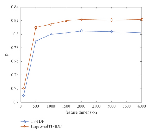
The following information can be seen in the experimental findings given in Figure 3. (1) The classification result P value is low when the feature dimension is tiny. (2) The P value of the classification result exhibits a trend of increase as the feature dimension increases. (3) When the feature size is small, the P value rises quickly, but when the feature dimension is high, the P value increases slowly until it plateaus. (4) The revised TF-IDF method has a higher P value than the traditional TF-IDF technique. The improved TF-IDF algorithm in this work has a significant improvement over the other two algorithms, and the P value of the better TF-IDF algorithm is always high, regardless of the number of feature dimensions. When compared to TF-IDF, the revised TF-IDF algorithm has a P value improvement of 2.2 percent in each feature dimension.

The experimental result (1) reveals that when the feature dimension is small, the expressive ability of the feature to the sample is insufficient to properly reflect the difference between the samples, making learning the difference between the samples difficult for the classification algorithm. (2) It is indicated that when the feature dimension grows, the feature becomes more representative of the sample and can better discriminate the sample, resulting in an increase in the P value of the classification model. (3) It is indicated that when the feature dimension is small, adding a given dimension improves the classification model’s performance more noticeably; however, when the feature dimension is large, adding the same dimension has less of an impact on the classification model’s performance. The modified TF-IDF is more discriminative for samples under multiple feature dimensions than the other two feature weight methods; hence the classification model’s P value is larger.

4.3. Feature Selection and Feature Weight Selection Experiments

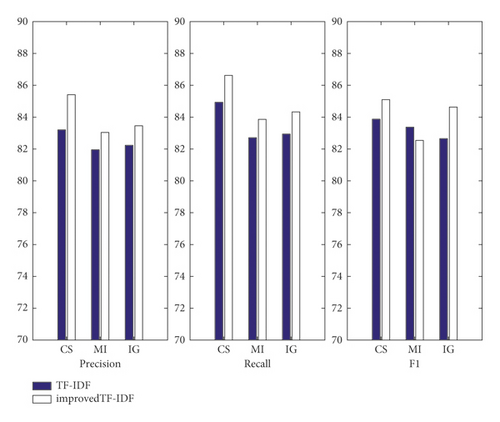
The feature dimension chosen in this paper is 1500, as determined by the feature dimension experiment. This research uses three feature selections: chi-square statistics, mutual information, and information gain, to see which feature selection and feature weight algorithm are best for text literature classification algorithm. The original TF-IDF method and the improved TF-IDF method are used in the feature weight algorithm. The classifier employs RF and has a total of four categories. Table 2 displays the outcomes of the experiments.

2. Experimental results of different feature selection and feature weight algorithms.

Feature selection algorithm	Feature weight algorithm	P/%	R%	F1/%
Chi-square statistics (CS)	TF-IDF	83.20	84.93	83.87
Chi-square statistics (CS)	Improved TF-IDF	85.41	86.62	85.10

Mutual information (MI)	TF-IDF	81.95	82.71	83.37
Mutual information (MI)	Improved TF-IDF	83.04	83.86	82.54

Information gain (IG)	TF-IDF	82.23	82.94	82.65
Information gain (IG)	Improved TF-IDF	83.46	84.33	84.63

When the data in Table 2 and Figure 4 are compared, the following is discovered: (1) The TF-IDF algorithm is paired with the three feature selection algorithms; the classification model’s average accuracy, average recall, and average F1 value are all at the lowest level. The precision value of the modified TF-IDF algorithm has increased by an average of 2% when compared to the TF-IDF algorithm. (2) The chi-square statistical performance is somewhat better compared to three other feature selection algorithms, regardless of whether feature weight method is combined, which is consistent with the research results of many researchers.

4.4. Classifier Selection Experiment

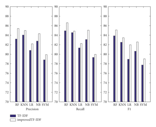
Based on the above experimental results, this paper determines that the feature selection algorithm in the literary text classification task is chi-square statistics, and the feature dimension is 1500. RF [19], K-nearest neighbor algorithm (KNN) [20], Logistic Regression (LR) [21], Naive Bayes (NB) [22], and SVM [23] were combined with TF-IDF and improved TF-IDF algorithm for comparison experiments, and the experimental results are shown in Table 3.

3. Experimental results obtained by different classifiers.

Classifiers	Feature weight algorithm	P/%	R/%	F1/%
RF	TF-IDF	83.20	84.93	83.87
RF	Improved TF-IDF	85.41	86.62	85.10

KNN	TF-IDF	84.04	84.55	82.52
KNN	Improved TF-IDF	84.98	84.86	83.47

LR	TF-IDF	80.82	81.33	78.95
LR	Improved TF-IDF	82.19	82.25	81.98

NB	TF-IDF	82.77	83.10	80.64
NB	Improved TF-IDF	84.32	85.06	82.58

SVM	TF-IDF	78.83	79.34	77.75
SVM	Improved TF-IDF	79.92	79.98	79.03

Figure 5 indicates that the RF classifier works best when employing the TF-IDF algorithm or the improved TF-IDF approach, with precision values of 83.2 percent and 85.41 percent, respectively. Because the support vector machine is a binary classification technique, its classification effect is weak, and multiclassification is frequently based on binary classification utilizing one-to-many, one-to-one, or hierarchical support approaches. The upgraded TF-IDF algorithm performs better than the original TF-IDF algorithm in classification. Precision, recall, and F1 have all been improved with an average increase of 1.8 percent using the improved TF-IDF algorithm proposed in this article, demonstrating the importance of the better TF-IDF method proposed in this work.

5. Conclusion

With the generation of massive literary texts, how can literary texts be efficiently saved while also providing users with a quick retrieval method? To address this issue, many Internet texts must be classified and sorted in order to facilitate information management and extraction. As a result, automatic text classification technology is being developed. It is both an urgent need and a very promising research direction. A strategy for quickly and efficiently categorizing literary works is proposed in this paper. The TF-IDF technique is one of the most extensively used text classification algorithms. Accordingly, the TF-IDF algorithm in this paper’s application scenario does not help improve classification accuracy because it uses the relationship between the feature words and the number of texts they appear in while ignoring the difference in feature word distribution between different categories. This paper proposes an improved TF-IDF algorithm for the problem of feature words appearing in different disciplines with different frequencies and meanings in different disciplines, with the goal of classification of literary texts. To distinguish features, the existing discipline classification is used as a reference. The meaning of words in various disciplines is to boost confidence in the TF-IDF algorithm’s results. An improved TF-IDF algorithm proposed in this paper has been shown to not only improve the performance of text classification but also improve the generalization and robustness of the algorithm by conducting comparative experiments on feature dimension selection and algorithms for selecting features, as well as the classifier. The proposed method can be implemented in the market. However, there are still some areas for improvement in this study, such as the effect on imbalanced datasets, which is less than ideal. This will be the focus of future research.

Conflicts of Interest

The author declares no conflicts of interest.

Acknowledgments

This work was supported by the Hubei University of Police.

Open Research

Data Availability

The labeled datasets used to support the findings of this study are available from the corresponding author upon request.

References

1 Luhn H. P., The automatic creation of literature abstracts, IBM Journal of Research and Development. (1958) 2, no. 2, 159–165, https://doi.org/10.1147/rd.22.0159.
10.1147/rd.22.0159
Web of Science® Google Scholar
2 Selva Birunda S. and Kanniga Devi R., A review on word embedding techniques for text classification, Innovative Data Communication Technologies and Application. (2021) 59, 267–281, https://doi.org/10.1007/978-981-15-9651-3_23.
10.1007/978-981-15-9651-3_23
Google Scholar
3 Maron M. E. and Kuhns J. L., On relevance, probabilistic indexing and information retrieval, Journal of the ACM. (1960) 7, no. 3, 216–244, https://doi.org/10.1145/321033.321035, 2-s2.0-84945708697.
10.1145/321033.321035
Web of Science® Google Scholar
4 Ganiz M. C., George C., and Pottenger W. M., Higher order naïve bayes: a novel non-IID approach to text classification, IEEE Transactions on Knowledge and Data Engineering. (2011) 23, no. 7, 1022–1034, https://doi.org/10.1109/tkde.2010.160, 2-s2.0-80054909897.
10.1109/TKDE.2010.160
Web of Science® Google Scholar
5 Guo Y., Yu L., Wen Z., and Li M., Using support vector machine combined with auto covariance to predict protein-protein interactions from protein sequences, Nucleic Acids Research. (2008) 36, no. 9, 3025–3030, https://doi.org/10.1093/nar/gkn159, 2-s2.0-44349159560.
10.1093/nar/gkn159
CAS PubMed Web of Science® Google Scholar
6 Minaee S., Kalchbrenner N., Cambria E., Nikzad N., Chenaghlu M., and Gao J., Deep learning--based text classification, ACM Computing Surveys. (2021) 54, no. 3, 1–40, https://doi.org/10.1145/3439726.
10.1145/3439726
Web of Science® Google Scholar
7 Akpatsa S. K., Li X., and Lei H., A survey and future perspectives of hybrid deep learning models for text classification, Lecture Notes in Computer Science. (2021) 12736, 358–369, https://doi.org/10.1007/978-3-030-78609-0_31.
10.1007/978-3-030-78609-0_31
Google Scholar
8 Yong Z., Youwen L., and Shixiong X., An improved KNN text classification algorithm based on clustering, Journal of Computers. (2009) 4, no. 3, 230–237.
Google Scholar
9 Joachims T., Text categorization with support vector machines: learning with many relevant features, Proceedings of the European Conference on Machine Learning, 1998, Berlin, Heidelberg, Springer, 137–142, https://doi.org/10.1007/bfb0026683.
10.1007/bfb0026683
Google Scholar
10 Chen T. and Guestrin C., XGBoost: a scalable tree boosting system, Proceedings of the 22nd ACM SIGKDD International Conference on Knowledge Discovery and Data Mining, August 2016, San Francisco, USA, ACM, 785–794.
Google Scholar
11 Ke G., Meng Q., Finley T., Wang T., Chen W., Ma W. et al., LightGBM: a highly efficient gradient boosting decision tree, Proceedings of the Advances in Neural Information Processing Systems, December 2017, Long Beach, CA, USA, 3146–3154.
Google Scholar
12 Prokhorenkova L., Gusev G., Vorobev A., Dorogush A. V., and Gulin A., CatBoost: unbiased boosting with cate gorical features, Proceedings of the 32nd International Conference on Neural Information Processing Systems, December 2018, Montréal, Canada, 6639–6649.
Google Scholar
13 Nigam K., McCallum K. A., Thrun S., and Mitchell T., Text classification from labeled and unlabeled documents using EM, Machine Learning. (2000) 39, no. 2-3, 103–134, https://doi.org/10.1023/a:1007692713085.
10.1023/A:1007692713085
Web of Science® Google Scholar
14 Collobert R., Weston J., Bottou L., Karlen M., Kavukcuoglu K., and Kuksa P., Natural lan gauge processing (almost) from scratch, Journal of Machine Learning Research. (2011) 12, no. Aug, 2493–2537.
Web of Science® Google Scholar
15 LeCun Y., Bottou L., Bengio Y., and Haffner P., Gradient-based learning applied to document recognition, Proceedings of the IEEE. (1998) 86, no. 11, 2278–2324, https://doi.org/10.1109/5.726791, 2-s2.0-0032203257.
10.1109/5.726791
Web of Science® Google Scholar
16 Kolen F. J. and Kreme C. S., Gradient flow in recurent nets: the difficulty of learning LongTerm dependencies, Proceedings of the IEEE. (2009) 62, no. 14, 1205–1222.
Google Scholar
17 Hochreiter S. and Schmidhuber J., Long short-term memory, Neural Computation. (1997) 9, no. 8, 1735–1780, https://doi.org/10.1162/neco.1997.9.8.1735, 2-s2.0-0031573117.
10.1162/neco.1997.9.8.1735
CAS PubMed Web of Science® Google Scholar
18 Zhou C., Sun C., Liu Z., and Lau F. C. M., A C-LSTM neural network for text classification, Computer Science. (2015) 1, no. 4, 39–44.
Google Scholar
19 Salles T., Gonçalves M., Rodrigues V., and Rocha L., Improving random forests by neighborhood projection for effective text classification, Information Systems. (2018) 77, 1–21, https://doi.org/10.1016/j.is.2018.05.006, 2-s2.0-85048563895.
10.1016/j.is.2018.05.006
Web of Science® Google Scholar
20 Prasanti A. A., Fauzi M. A., and Furqon M. T., Neighbor weighted K-nearest neighbor for s online classification, Indonesian Journal of Electrical Engineering and Computer Science. (2018) 12, no. 1, 155–160, https://doi.org/10.11591/ijeecs.v12.i1.pp155-160, 2-s2.0-85051276771.
10.11591/ijeecs.v12.i1.pp155-160
Google Scholar
21 Jurka T. P., maxent: an R package for low-memory multinomial logistic regression with support for semi-automated text classification, R Journal.(2012) 4, no. 1, 56–59.
10.32614/RJ-2012-007
Web of Science® Google Scholar
22 Yaremenko V. S., Rogoza W. S., and Spitkovskyi V. I., Application of neural network algorithms and naive bayes for text classification, Journal of Theoretical and Applied Information Technology. (2021) 99, no. 1, 125–134.
Google Scholar
23 Wen Z., Yoshida T., and Tang X., Text classification based on multi-word with support vector machine, Knowledge-BAsed Systems. (2008) 21, no. 8, 879–886.
10.1016/j.knosys.2008.03.044
Web of Science® Google Scholar

Citing Literature

All articles

Application of an Improved TF-IDF Method in Literary Text Classification

Abstract

1. Introduction