In order to improve the effect of UAV intelligent control, this paper will improve machine vision technology. Moreover, this paper adds scale information on the basis of the LSD algorithm, uses the multiline segment standard to merge these candidate line segments for intelligent recognition, and uses the LSD detection algorithm to improve the operating efficiency of the UAV control system and reduce the computational complexity. In addition, this paper combines machine vision technology and multiagent decision-making technology for UAV intelligent control and builds an intelligent control system, which uses intelligent machine vision technology for recognition and multiagent decision-making technology for motion control. The research results show that the UAV intelligent control system based on machine vision and multiagent decision-making proposed in this paper can achieve reliable control of UAVs and improve the work efficiency of UAVs.

1. Introduction

Unmanned aerial vehicles can complete flight missions through wireless remote control or even autonomous control. Compared with ordinary manned aircraft, UAV has many advantages such as simple structure, flexible operation, low cost, easy manufacturing, and easy maintenance [1]. At the same time, the UAV can be remotely controlled by wireless equipment and will not endanger the life and safety of the operator in an accident [2]. Therefore, UAVs are widely used in various fields such as civil and military. In civil use, UAVs can be used for air transportation, remote aerial photography, traffic patrol, water conservancy monitoring, and forest fire fighting [3]. In the military, UAVs can be used for enemy reconnaissance, electronic interference, target positioning, and precise strikes on specific targets. According to the different body structures, UAV can be divided into two categories: fixed wing and rotary wing. Fixed-wing UAVs mainly include two types: propeller type and jet type. The principle is to use the thrust or pulling force generated by the engine to make the aircraft fly horizontally while using the lift generated by the wings to maintain the vertical motion of the body. Rotor UAVs are divided into two types: single-rotor and multirotor, and common multirotor UAVs have four-rotor, six-rotor, and eight-rotor forms. Single-rotor UAVs generally need a separate tail to balance the torque generated by the main wing, while multirotor UAVs can cancel each other’s rotation torque due to the opposite rotation of adjacent wings [4]. Therefore, the structure of the multirotor UAVs will be simpler, and the maneuverability will be more superior.

This paper combines machine vision technology and multiagent decision-making technology to study the intelligent control of UAVs, uses intelligent machine vision technology for recognition, and uses multiagent decision-making technology for motion control to improve the motion effect of UAVs.

2. Related Work

Intelligent control belongs to the advanced stage of the development of control theory. The use of intelligent control methods can solve the control problems of some complex systems that cannot be handled by traditional control methods. Different from the traditional control method, which relies heavily on the precise mathematical model of the controlled object [5], the intelligent control method can be applied to the control of uncertain objects with unknown models or model parameters and structural changes. At the same time, the intelligent control method also has good advantages for the control of systems with strong nonlinearity and complex tasks. With the continuous improvement and development of intelligent control theory, intelligent control has been successfully applied in many engineering fields and has become one of the most attractive and valuable technologies in the field of control technology. Rotor UAVs have complex structures and strong coupling between different axes, making it difficult to obtain accurate mathematical models. This is where intelligent control methods are good. The application of intelligent control methods to the attitude control of rotary wing drones can make up for the shortcomings of traditional control methods and improve control performance. In recent years, more and more scholars have begun to pay attention to the application of intelligent control methods in the attitude control of rotor drones, trying to improve the effect of rotor drone attitude control and truly realize intelligent control. Commonly used intelligent control methods include fuzzy control, neural network control, genetic algorithm, and ant colony algorithm. Fuzzy control is based on fuzzy set theory, fuzzy linguistic variables, and fuzzy logic reasoning and simulates human approximate reasoning and decision-making process [6]. The core part of the fuzzy control method is the determination of fuzzy rules. Generally speaking, fuzzy rules can be determined based on expert experience or experiments [7]. Literature [8] took the three-degree-of-freedom helicopter system as the research object, respectively, designed PID controller, LQR controller, and fuzzy controller to control the helicopter’s attitude, and compared the control effects of the three controllers through simulation and verified the fuzzy. The advantages of control: Literature [9] designed an intelligent four-rotor control system based on fuzzy logic. Literature [10] designed four fuzzy controllers for altitude, pitch angle, yaw angle, and tilt angle. The structures of these fuzzy controllers are all relatively simple, the fuzzy rules are determined by expert experience, and then the outputs of the four fuzzy controllers are used as the reference values of the driving voltages of the four motors to control the attitude of the quadrotor. Finally, the effectiveness of the control method is verified by simulation. Literature [11] takes into account the influence of air resistance and rotational torque on the quadrotor, establishes a dynamic model, and then uses a fuzzy control method to adjust the parameters of the PID controller. The design of the fuzzy controller is to find the input deviation, the deviation change rate and for the relationship between the three parameters of PID, the fuzzy controller designed a total of 49 fuzzy rules, and then the simulation verified that the control method has a better control effect. The neural network is a way of simulating human thinking. Although the structure of a single neuron is relatively simple and its functions are limited, the behavior that can be achieved by a network system composed of a large number of neurons is extremely colorful [12]. With the deepening of neural network control research, this method has become an important branch of intelligent control, and it has a wide range of applications in solving complex nonlinear, time-varying, and uncertain system control problems. Compared with traditional control methods, the research of neural network algorithms in the attitude control of rotary wing UAV is in its infancy [13]. In the control of rotary wing UAV, the neural network is often used to identify some unknown parameters to supplement and optimize traditional control methods such as PID, LQR, etc. Literature [14] designed a neural network. The PID control system has designed three neural networks for pitch angle, yaw angle, and roll angle. PID controller: the input of each neural network is the error of the corresponding attitude angle and the rate of change of the error, and the output is the correction value of the three parameters of the PID controller. The entire network adopts a four-layer neural network structure. Unfortunately, they did not give the training process of the neural network but only the network parameters after the training. Finally, the simulation demonstrated the superiority of the design method and other traditional methods in the control performance and carried out the method on the real object. The experiment verified the feasibility of the method. Literature [15] uses a neural network to modify PID parameters and gives the training process of a neural network based on ideal experimental data. Literature [16] designed a quadrotor control method based on neural network output feedback for the complex situation of the quadrotor in an outdoor environment. This method first designed a multilayer neural network to learn the dynamic characteristics of UAV online, and then a neural network is designed to provide feedback on the position and attitude of the UAV as well as external interference, and finally, the feedback information is sent to the feedback controller for control. Literature [17] verifies the convergence of the main parameters of the system and analyzes it through simulation experiments. The control performance of the strategy: Literature [18] proposed a robust adaptive controller based on radial neural network interference compensation for the symmetrical structure of the six-rotor attitude control problem, and the simulation verified the method’s suppression effect on interference. Literature [19] proposed a PIDNN control method combining neural network ideas and PID principles. Since then, many scholars have applied the method to the attitude control of three-degree-of-freedom helicopters and quadrotors. Simulations have verified that the method is relative to the effectiveness of PID control methods.

3. Intelligent Machine Vision Optical Inspection Algorithm

LSD (Line Segment Detector) is a linear timeline segment detector that can provide subpixel accuracy results. It can process any digital image without any parameter adjustment, and at the same time, it can control the number of its own error detection: on average, each image allows one error alarm. Compared with the classic Hough transform, the LSD line segment detection algorithm not only improves the accuracy but also greatly reduces the computational complexity and greatly improves the speed.

The flow of the entire algorithm is roughly as follows:

(1)
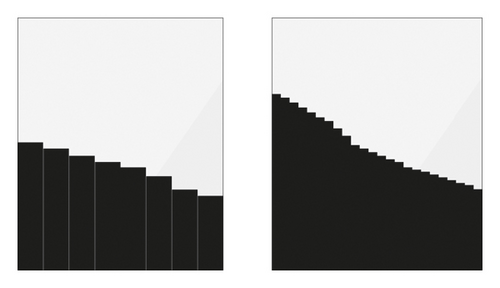
The algorithm reduces the image to 80% of the original through Gaussian downsampling (both the length and width are reduced to 80% of the original, and the total pixels become 64% of the original). The purpose of this is to reduce or eliminate the aliasing effect that often appears in the image, as shown in Figure 1:
(2)
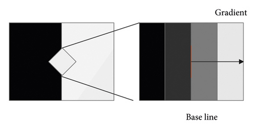
The algorithm calculates the gradient amplitude and gradient angle of each pixel in the image, as shown in Figure 2. The algorithm uses a 2 × 2 template to calculate the gradient and gradient angle. The smallest possible template is used to reduce the dependence between pixels in the gradient calculation process while maintaining a certain degree of independence. We assume that i (x, y) is the image gray value at pixel (x, y); the gradient calculation formula is as follows:
(1)
The gradient angle calculation formula is as follows:
(2)
The gradient amplitude calculation formula is as follows [20]:
(3)
(3)
The algorithm uses a greedy algorithm to pseudosort the gradient magnitudes calculated in the second step. If a normal sorting algorithm processes n data, the time complexity of pseudosorting is linear, which can save time to a certain extent. Pseudosorting is to divide the obtained gradient amplitude range (0–255) into 1024 levels, each gradient amplitude is divided into a level, and the same gradient amplitude is divided into the same level. At the same time, a state table is established, all pixels are set to UNUSED, and then the state corresponding to the pixels whose gradient amplitude is less than is set to USED. Among them, there are the following:
(4)
In the above formula, q represents the error boundary that may occur in the gradient quantization process. According to the empirical value, q is set to 2. τ represents the angle tolerance in the fourth step of the area growth algorithm and is usually set to 22.5°.
(4)
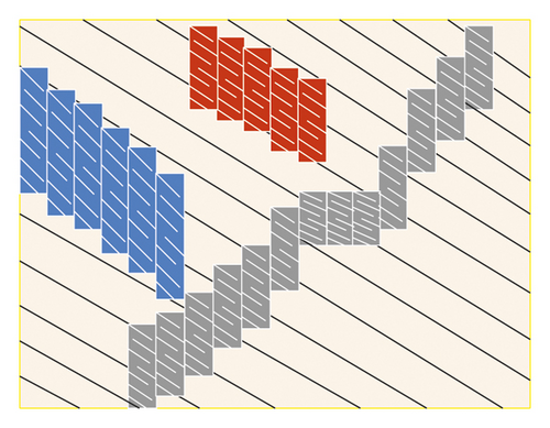
The algorithm uses the area growth algorithm to generate the line segment support area, as shown in Figure 3. The algorithm first takes the pixel with the largest gradient amplitude as the seed point (we usually think that the higher the gradient amplitude, the stronger the edge) and then searches for the pixel with the state of UNUSED in the neighborhood of the seed point. If the absolute value of the difference between the gradient angle and the area angle is between 0-τ, the pixel is added to the area. Here, the initial area angle is the gradient angle of the seed point. Each time a new pixel is added to the area, the area angle needs to be updated.
The formula for updating the area angle is as follows:
(5)
Among them, θ_j represents the gradient angle of the pixel j in the area, and then the process is repeated until no pixels can be added to the area.
(5)
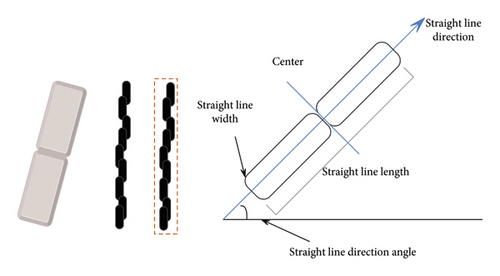
The algorithm estimates the rectangle of the line segment support area calculated in the fourth step. The result of the fourth step calculation is a series of adjacent discrete points; therefore, they need to be contained in a rectangular box r (the rectangle is the candidate of the line segment), as shown in Figure 4. The size of the rectangle is mainly selected to cover the entire area, that is, the smallest rectangle that can contain the area supported by the line segment. Obviously, this rectangular frame r contains not only the points in the line segment support area, which are also called alignment points but also includes the points close to the line segment support area, which do not belong to the outer points. The center coordinates of the rectangle are as follows [21]:
(6)
Among them, G(j) is the gradient magnitude of the pixel j, and the main direction of the rectangle is set as the angle of the eigenvector corresponding to the smallest eigenvalue of the matrix.
(6)
The algorithm verifies whether the candidate rectangle is a straight line segment by calculating the Number of False Alarms (NFA). The calculation formula of NFA is as follows:
(7)

Details are in the caption following the image — Open in figure viewer PowerPoint

Here, N_test refers to the number of potential rectangular boxes with an image size of M^∗N:

(8)

Among them, k(r, I) is the number of alignment points in the rectangle r in the contrast model (refers to the hypothetical perfect noise image model, the characteristic of this model is that the gradient angles are randomly distributed independently and evenly distributed in [0 ~ 2π]), and k(r, i) is the number of alignment points in the rectangle r at the same position in the image i to be detected. Here, the false alarm number NFA represents the probability that the number of alignment points in a certain candidate rectangle r in the image to be detected is less than the number of alignment points in the same position r in the control model. The larger the NFA is, the more similar the current r is to the same position r in the control model, and the less likely it is to be a straight line target for detection; on the contrary, the more likely it is to be a straight line. We also know the following [22]:

(9)

B(n, k, p) represents the binomial distribution, as shown below:

(10)

n represents the total number of pixels in the rectangle r, k represents the number of alignment points in the rectangle r in the image i to be detected, and p represents the probability that the pixel points in the control model are aligned points, as shown below [23]:

(11)

Therefore, the NFA of a matrix r is finally obtained as follows:

(12)

If NFA(r) ≤ ε, the rectangular area is considered to be a straight line, which ε is set to 1. Here, the threshold can be changed, and there is no significant difference in the detection results, so we uniformly use the threshold value of 1.

In the LSD algorithm, we assume the angle threshold δ of the line segment L, then the NFA of the line segment L is defined as follows:

(13)

Among them, χ is a normalized value, N is the number of potential line segments in the image to be detected, B is the binomial distribution, n is the total number of pixels in the line segment L, k represents the number of alignment points in the line segment L, and p refers to the probability that a random pixel is an alignment point. When and only if NFA(L) is less than a given threshold, the line segment L is considered to be meaningful.

On the basis of the LSD algorithm, the algorithm adds scale information; that is, the algorithm first finds a longer line segment on a coarse scale and then further refines its position on a finer scale. At each scale, new line segment candidates are still considered for the same position instead of just using the line segment detected by the previous scale and then using the multiline segment criterion to merge these candidate line segments. The original image is denoted as I, and the length and width of the image are reduced by 1/2ⁿ , respectively, as shown below:

(14)

I represents the finest scale, which is the original image. The larger the nthe thicker the scale. The maximum value of n depends on whether the length or width of the Iⁿ image is one of the pixel values below 500. If it is lower than 500, the scale is no longer reduced. The algorithm first uses the LSD algorithm to detect line segments on the coarse scale. We assume that the line segment Lⁿ is detected in the coarse-scale image Iⁿ, the line segment direction is denoted as θ(Lⁿ), and the given angle threshold is δⁿ. We define Sⁿ⁻¹ as the rectangular area corresponding to Lⁿ enlarged in the fine-scale image Iⁿ⁻¹. We denote Rⁿ⁻¹ as a subset of pixels in Sⁿ⁻¹ where the gradient direction of the pixel and the angle difference between the direction of the line segment Lⁿ are lower than the threshold δⁿ, as shown below:

(15)

Then, the algorithm calculates a set Eⁿ⁻¹, which includes all the connected components in Rⁿ⁻¹, thus generating potential new line segments. These components may belong to the same line segment, may be parallel to each other, or close to the same line segment. They are fused together in the coarse-scale image and are judged as a line segment.

We assume that n line segments S = {s₁, …, s_n} are given, and $L$ is the best line segment calculated from the line segment set s_i. The rectangle corresponding to this line segment refers to the smallest rectangle that contains the rectangles associated with all line segments s_i. The corresponding fusion score of this group of line segments is defined as follows:

(16)

If the fusion score is positive, it means that NFA_M is lower than the NFA of a single line segment, so it should be merged. This defines a line segment merging standard that does not depend on any parameters and thus has an adaptive characteristic.

In fact, the set Eⁿ⁻¹ contains many temporary line segments, and there are countless combinations of these temporary line segments, which we cannot test one by one. Therefore, it can be iterated by a greedy algorithm. The algorithm first selects the smallest NFA component e from the set Eⁿ⁻¹and then uses e as the benchmark to calculate all other components that are fully aligned with it, as shown below:

(17)

Among them, l(e) is a line segment passing through the center of component e, the angle is θ(e), l(e^′) is a line segment passing through the center of component e^′, and the angle is θ(e^′). Then, the algorithm calculates the fusion score calculation method of C(e) as shown in equation (16). If it is positive, the algorithm replaces the subline segments in C(e) with the merged version of C(e). It continues to iterate until all the temporary segments in Eⁿ⁻¹ have been tested.

Finally, the algorithm calculates the NFA of all the line segments, leaving only the meaningful ones. When there is noise or the contrast is low, the line segment Lⁿ detected in the coarse-scale image usually does not meet the NFA condition. Therefore, it is often impossible to derive the line segment in the fine-scale image. In this case, the original line segment in the coarse scale is directly retained, and no more attempts are made to find a finer line segment at the same position in the fine-scale image, and the line segment is extracted only at this scale using LSD.

The algorithm first matches all the line segments in L_i with all the line segments in L_j to generate a potential corresponding relationship, where L_i refers to the line segment detected in image I_i, L_j refers to the line segment detected in image I_j, and I_i and I_j are two images to be matched. For specific line segment pairs,

. The algorithm first calculates the epipolar lines corresponding to the end points of the line segment, such as the extreme lines of the end points

and

in the image I_j. The algorithm intersects

and these two polar lines and obtains two intersection points x_p and x_q, and the two end points

and V of x_p and x_q are collinear with

, and then defines a matching score between the line segments Z and X, as shown below:

(18)

Among them, inner ({…}) and outer ({…}), respectively, represent the Euclidean distance corresponding to a pair of outer points and a pair of inner points among the four collinear points. (18) illustrates the degree of matching between two two-dimensional line segments. If all the line segments can be detected ideally, that is, no occlusion, not too long, and not too short, then the matching score will be exactly 1. Therefore, in general, if the matching score is greater than a fixed threshold, it is considered that there is a potential matching correspondence between the line segments and .

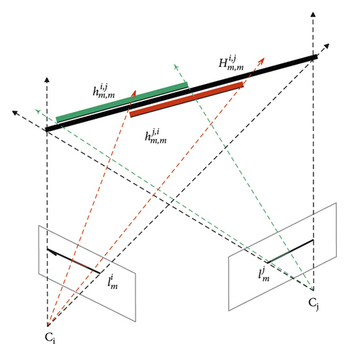
Knowing all the camera poses, we can use the camera pose to project each two-dimensional corresponding relationship into the three-dimensional space to get a three-dimensional line segment hypothesis. For example, the algorithm transforms the two-dimensional correspondence relationship to the three-dimensional line segment , where is the intersection of the plane formed by the camera center C_i, C_j ∈ R³ and the two-dimensional line segments and . For each corresponding relationship, calculate two three-dimensional line segment hypotheses , respectively, and they all fall on the three-dimensional line segment , where the end points of the back projection of and coincide with the end points of and , respectively. Similar to a two-dimensional line segment, a three-dimensional line segment is also composed of two three-dimensional end points . Note that . Usually, due to occlusion and inaccurate two-dimensional line segment detection, . However, the line segments and are always collinear with the infinite line segment . Then, by analyzing the spatial consistency of the three-dimensional line segment hypothesis, the correct match can be selected from the incorrect matching line segments. The hypothesis of the three-dimensional line segment generated by the two-dimensional potential matching line segment is shown in Figure 5.

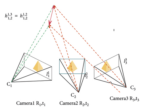
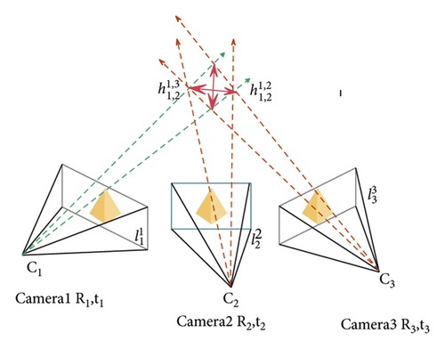
Next, we need to calculate the confidence of each pair of matching line segments between all images and all of their neighbors. The algorithm judges whether the three-dimensional hypothesis generated by the line segment and the line segment is reasonable through the confidence, that is, whether the three-dimensional hypothesis is suitable for all matching images (except for the matching of I_i and I_j). We assume that the line segment in image I_i and the line segment in image I_j have been correctly matched, and the other line segment in image I_b has been correctly matched, then the 3D hypotheses calculated from lines and and the 3D hypotheses calculated from and should be very close to each other in space as shown in Figure 6 (in the ideal noise-free case, they should be perfectly colinear). On the contrary, if the matching is incorrect, the three-dimensional hypothesis obtained cannot be spatially close to that shown in Figure 7. This is because the wrong assumptions obtained by triangulation are not geometrically consistent. However, the correct assumptions obtained by triangulation always support each other. Therefore, this feature of geometric consistency can be used to eliminate mismatches.

To measure the similarity based on the spatial distance and angular error between two three-dimensional hypotheses, we first define confidence for a corresponding relationship

, as shown below:

(19)

Among them, the A calculation is derived from the correlation between two three-dimensional hypotheses of the same two-dimensional line segment

. This correlation is defined as follows:

(20)

S^a is the angle similarity in the three-dimensional line segment hypothesis, and $S^(d)$ is the position similarity in the three-dimensional line segment hypothesis, which is defined as follows:

(21)

Among them, ∠(h₁, h₂) represents the angle between two line segments (in degrees), l_⊥(Z, h₂) is the vertical distance between the three-dimensional point Z and the straight line passing through h₂, and is the Euclidean distance between the camera center C_i of the image I_i and the three-dimensional point Z, that is, the depth of the three-dimensional point Z along the optical axis of the camera. In order to prevent only a few weak supporters, the confidence is also high. We cut the correlation and only accept the values above 1/2.

Using the depth-adaptive spatial regularization function

, this regularization function is defined as follows:

(22)

This is a linear function of depth d. The slope μ/d_med of this function is composed of the specified spatial regularization factor μ (for example, 5 cm of the reconstruction result corresponds to 0.05) and the regularization depth d_med. In this paper, d_med simply refers to the distance from the world point to the camera. However, this formula needs to know the reconstruction scale information in advance (the decision of μ requires scale information). The fact is that the size information of obstacles is often not known. Therefore, a formula with a constant scale is used to deal with this situation, as shown below:

(23)

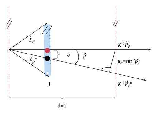
This is also a linear function of depth d. However, this time the slope μ_σ is derived from the geometric mechanism of the camera. We assume that given a standard pinhole camera model, move the origin horizontally by a regularized σ pixel to obtain (∼ represents homogeneous coordinates), and then calculate the angle β between the two three-dimensional rays and , where K⁻¹ is the internal parameter matrix of the camera.

Then, the algorithm simply calculates μ_σ = sin(β), which is basically the maximum distance to move the origin of the camera at depth d = 1, so that the distance between the reprojection of the moving point and the midpoint of the image is less than or equal to σ, as shown in Figure 8. This formula ensures that when the corresponding 3D line segment is assumed to be far away from the camera, the greater the distance from the 3D point to the line segment, the less the penalty, and vice versa. Therefore, in order to maintain scale invariance, the new is used instead of σ_p(d) here.

It is now possible to determine whether a matching three-dimensional line segment hypothesis makes sense. Only when , this assumption is retained for further processing, which means that at least two line segments from two additional images (except I_i and I_j) support . Therefore, a set of sparser correspondences can be finally obtained, and most of the mismatches are removed.

4. UAV Intelligent Control Based on Machine Vision and Multiagent Decision-Making

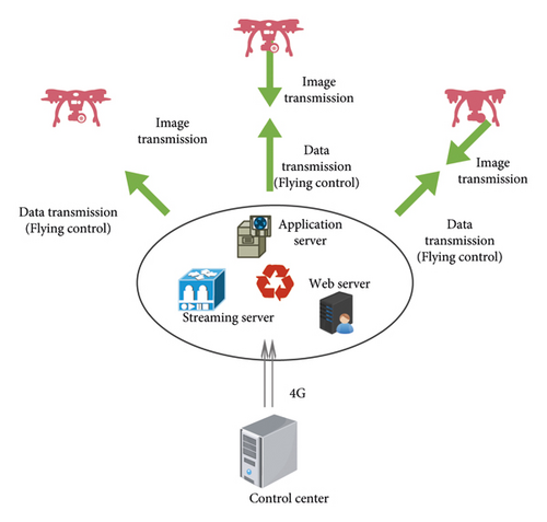
The intelligent control process of UAV based on machine vision and multiagent decision-making is shown in Figure 9. When traditional UAVs operate remotely, they need to carry ground station equipment. Usually, a ground station device can only control one drone at a time, and the ground station and the command center can transmit data through the 5G network. When UAV operations are carried out through the intelligent control of drones based on machine vision and multiagent decision-making, there is no need to carry special ground station equipment, and the functions of the ground station software are deployed on the cloud platform. This effectively reduces the cost of system hardware while obtaining the powerful computing power of cloud computing. In addition, different from the one-to-one matching of UAVs and ground stations in the traditional way, in the UAV intelligent control system based on machine vision and multiagent decision-making, each UAV is a node of the system, and the UAV can be identified through the network address, and multiple UAVs can be controlled at the same time.

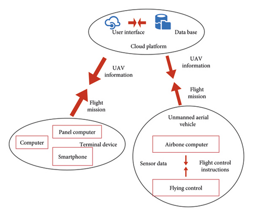
In order to improve the efficiency of multiagent decision-making, this paper proposes to carry out intelligent control data transmission and processing on the cloud platform. The UAV cloud control scheme proposed in this paper is shown in Figure 10, which mainly includes three parts: terminal equipment, cloud platform, and UAV.

After constructing the above model, the model of this paper is tested and researched. The model in this paper uses machine vision for intelligent recognition and performs intelligent control of UAVs under the support of multiagent decision-making. Therefore, this paper uses intelligent machine vision to recognize UAV images, and the results are shown in Table 1.

1. Machine vision effect detection.

Number	Machine vision
1	93.574
2	95.891
3	93.206
4	97.714
5	93.016
6	96.640
7	96.378
8	96.080
9	93.348
10	96.169
11	97.773
12	94.359
13	93.397
14	96.687
15	95.397
16	95.699
17	95.067
18	93.170
19	93.181
20	95.418
21	96.714
22	96.528
23	95.344
24	97.915
25	96.423
26	95.724
27	95.602
28	96.282
29	93.132
30	93.033
31	93.850
32	93.065
33	95.412
34	94.642
35	96.910
36	96.705
37	97.502
38	97.215
39	94.618
40	97.666
41	97.794
42	97.408
43	96.531
44	97.147
45	94.713
46	96.370
47	93.667
48	94.060
49	95.951
50	96.590
51	97.032
52	97.511
53	97.285
54	93.291
55	96.034
56	95.009
57	97.524

Based on the above detection, it can be seen that the machine vision method proposed in this paper performs better in UAV visual recognition. On this basis, the intelligent control effect of UAVs based on machine vision and multiagent decision-making can be verified, and the results shown in Table 2 below are obtained.

2. The control effect of the UAV intelligent control system based on machine vision and multiagent decision-making.

Number	Control effect
1	91.992
2	93.169
3	89.641
4	89.259
5	90.691
6	88.784
7	93.029
8	88.650
9	93.561
10	92.127
11	91.382
12	91.923
13	89.110
14	89.091
15	93.236
16	88.166
17	93.668
18	91.834
19	93.654
20	91.288
21	88.472
22	89.224
23	89.139
24	90.184
25	88.419
26	89.019
27	92.395
28	93.662
29	88.304
30	89.978
31	92.967
32	89.431
33	88.081
34	88.010
35	92.612
36	93.456
37	90.242
38	90.020
39	89.008
40	93.271
41	90.150
42	91.875
43	91.077
44	93.118
45	90.849
46	91.347
47	90.163
48	88.486
49	93.761
50	90.835
51	92.676
52	90.935
53	93.267
54	91.940
55	92.074
56	91.276
57	92.169

From the above research, it can be seen that the UAV intelligent control system based on machine vision and multiagent decision-making can achieve reliable control of UAVs and improve the work efficiency of UAVs.

5. Conclusion

The UAV flight control system is developed on the basis of manned aircraft, but in contrast, there are some new technical requirements. The primary function of the UAV flight control system is to enable the UAV to autonomously control the flight attitude, flight speed, and flight path. At the same time, the UAV flight control system needs to send a series of instructions to dispatch the various functional components of the aircraft during the flight of the aircraft, receive feedback information, and vote on redundant subsystems. Finally, when the aircraft system fails, the flight control system must have the ability to self-check the failure and restore the aircraft to normal flight through the aircraft redundancy system. This paper combines machine vision technology and multiagent decision-making technology to study the intelligent control of drones, uses intelligent machine vision technology for recognition, and uses multiagent decision-making technology for motion control to improve the motion effect of drones. The research shows that the UAV intelligent control system based on machine vision and multiagent decision-making proposed in this paper can achieve reliable control of UAVs and improve the work efficiency of UAVs.

Conflicts of Interest

The authors declare that they have no conflicts of interest.

Acknowledgments

This study was sponsored by the Hubei University of Technology.

Open Research

Data Availability

The labeled dataset used to support the findings of this study is available from the corresponding author upon request.

References

1 Duarte F. L. and De Lamare R. C., C-RAN-Type chd relaying with recursive maximum minimum distance, IEEE Communications Letters. (2020) 24, no. 11, 2623–2627, https://doi.org/10.1109/lcomm.2020.3009845.
10.1109/LCOMM.2020.3009845
Web of Science® Google Scholar
2 Hu L., Tian Y., Yang J., Taleb T., Xiang L., and Hao Y., Ready player one: UAV-Clustering-Based multi-task offloading for vehicular VR/AR gaming, IEEE Network. (2019) 33, no. 3, 42–48, https://doi.org/10.1109/mnet.2019.1800357, 2-s2.0-85068856934.
10.1109/MNET.2019.1800357
Web of Science® Google Scholar
3 Yi W., Liu Y., Bodanese E., Nallanathan A., and Karagiannidis G. K., A unified spatial framework for UAV-a networks, IEEE Transactions on Communications. (2019) 67, no. 12, 8801–8817, https://doi.org/10.1109/tcomm.2019.2945332.
10.1109/TCOMM.2019.2945332
Web of Science® Google Scholar
4 Feng W., Wang J., Chen Y., Wang X., Ge N., and Lu J., UAV-aided MIMO cit, IEEE Internet of Things Journal. (2019) 6, no. 2, 1731–1740, https://doi.org/10.1109/jiot.2018.2874531, 2-s2.0-85065606365.
10.1109/JIOT.2018.2874531
Web of Science® Google Scholar
5 He H., Zhang S., Zeng Y., and Zhang R., Joint altitude and bo-enabled multiuser communications, IEEE Communications Letters. (2018) 22, no. 2, 344–347, https://doi.org/10.1109/lcomm.2017.2772254, 2-s2.0-85034259558.
10.1109/LCOMM.2017.2772254
Web of Science® Google Scholar
6 Li B., Zhang S., Zhang X., Xi B., and Tian Y., Application and research of scheduling mechanism for UAV cluster launching control system, Xibei Gongye Daxue Xuebao/Journal of Northwestern Polytechnical University. (2018) 36, no. 2, 353–358, https://doi.org/10.1051/jnwpu/20183620353.
10.1051/jnwpu/20183620353
Google Scholar
7 Mei W., Wu Q., and Zhang R., Cellular-connected UAV: uplink association, power control and interference coordination, IEEE Transactions on Wireless Communications. (2019) 18, no. 11, 5380–5393, https://doi.org/10.1109/twc.2019.2936021.
10.1109/TWC.2019.2936021
Web of Science® Google Scholar
8 Zhu Q., Jiang K., Chen X., Zhong W., and Yang Y., A novel 3D non-stationary UAV-MIMO channel model and its statistical properties, China Communications. (2018) 15, no. 12, 147–158, https://doi.org/10.12676/j.cc.2018.12.012.
10.12676/j.cc.2018.12.012
Web of Science® Google Scholar
9 Wang X. and Gursoy M. C., Coverage analysis for energy-harvesting UAV-a cellular networks, IEEE Journal on Selected Areas in Communications. (2019) 37, no. 12, 2832–2850, https://doi.org/10.1109/jsac.2019.2947929.
10.1109/JSAC.2019.2947929
Web of Science® Google Scholar
10 Arafat M. Y. and Moh S., Localization and clustering based on swarm intelligence in UAV networks for emergency communications, IEEE Internet of Things Journal. (2019) 6, no. 5, 8958–8976, https://doi.org/10.1109/jiot.2019.2925567, 2-s2.0-85073460977.
10.1109/JIOT.2019.2925567
Web of Science® Google Scholar
11 Ebrahimi D., Sharafeddine S., Ho P. H., and Assi C., UAV-aided projection-based compressive data gathering in wireless sensor networks, IEEE Internet of Things Journal. (2019) 6, no. 2, 1893–1905, https://doi.org/10.1109/jiot.2018.2878834, 2-s2.0-85055868895.
10.1109/JIOT.2018.2878834
Web of Science® Google Scholar
12 Fu S., Tang Y., Zhang N., Zhao L., Wu S., and Jian X., Joint unmanned aerial vehicle (UAV) deployment and power control for internet of things networks, IEEE Transactions on Vehicular Technology. (2020) 69, no. 4, 4367–4378, https://doi.org/10.1109/tvt.2020.2975031.
10.1109/TVT.2020.2975031
Web of Science® Google Scholar
13 Liu D., Xu Y., Wang J., Chen J., Yao K., Wu Q., and Anpalagan A., Opportunistic UAV utilization in wireless networks: motivations, applications, and challenges, IEEE Communications Magazine. (2020) 58, no. 5, 62–68, https://doi.org/10.1109/mcom.001.1900687.
10.1109/MCOM.001.1900687
Web of Science® Google Scholar
14 Liu X., Liu Y., and Chen Y., Reinforcement learning in multiple-UAV networks: deployment and movement design, IEEE Transactions on Vehicular Technology. (2019) 68, no. 8, 8036–8049, https://doi.org/10.1109/tvt.2019.2922849.
10.1109/TVT.2019.2922849
Web of Science® Google Scholar
15 Yu T., Wang X., and Shami A., UAV-enabled spatial data sampling in large-scale IoT systems using da neural network, IEEE Internet of Things Journal. (2019) 6, no. 2, 1856–1865, https://doi.org/10.1109/jiot.2018.2876695, 2-s2.0-85055050513.
10.1109/JIOT.2018.2876695
Web of Science® Google Scholar
16 Wang Y. S., Hong Y. W. P., and Chen W. T., Trajectory learning, clustering, and user association for dynamically connectable UAV base stations, IEEE Transactions on Green Communications and Networking. (2020) 4, no. 4, 1091–1105, https://doi.org/10.1109/tgcn.2020.3005290.
10.1109/TGCN.2020.3005290
Google Scholar
17 Khabbaz M., Antoun J., and Assi C., Modeling and performance analysis of UAV-assisted vehicular networks, IEEE Transactions on Vehicular Technology. (2019) 68, no. 9, 8384–8396, https://doi.org/10.1109/tvt.2019.2911986.
10.1109/TVT.2019.2911986
Web of Science® Google Scholar
18 Liu D., Wang J., Xu K., Xu Y., Yang Y., Xu Y., Wu Q., and Anpalagan A., Task-driven relay assignment in distributed UAV communication networks, IEEE Transactions on Vehicular Technology. (2019) 68, no. 11, 11003, https://doi.org/10.1109/tvt.2019.2942095.
10.1109/TVT.2019.2942095
Web of Science® Google Scholar
19 Rahmaniar W. and Rakhmania A. E., Online digital image stabilization for an unmanned aerial vehicle (UAV), Journal of Robotics and Control (JRC). (2021) 2, no. 4, 234–239.
10.18196/jrc.2484
Google Scholar
20 Thibbotuwawa A., Bocewicz G., Nielsen P., and Zbigniew B., Planning deliveries with UAV routing under weather forecast and energy consumption constraints, IFAC-PapersOnLine. (2019) 52, no. 13, 820–825, https://doi.org/10.1016/j.ifacol.2019.11.231.
10.1016/j.ifacol.2019.11.231
Google Scholar
21 Motlagh N. H., Bagaa M., and Taleb T., UAV-based IoT platform: a crowd surveillance use case, IEEE Communications Magazine. (2017) 55, no. 2, 128–134, https://doi.org/10.1109/mcom.2017.1600587cm, 2-s2.0-85012979827.
10.1109/MCOM.2017.1600587CM
Web of Science® Google Scholar
22 Yu X., Dong X., Yang X., Chen C., Ruan L., Song F., and Gong Y., Air–ground integrated deployment for UAV enabled mobile edge computing: a hierarchical game approach, IET Communications. (2020) 14, no. 15, 2491–2499, https://doi.org/10.1049/iet-com.2019.1209.
10.1049/iet-com.2019.1209
Web of Science® Google Scholar
23 Liu X., Liu Y., Chen Y., and Hanzo L., Trajectory design and power control for multi-UAV assisted wireless networks: a machine learning approach, IEEE Transactions on Vehicular Technology. (2019) 68, no. 8, 7957–7969, https://doi.org/10.1109/tvt.2019.2920284.
10.1109/TVT.2019.2920284
Web of Science® Google Scholar

Citing Literature

All articles

UAV Intelligent Control Based on Machine Vision and Multiagent Decision-Making

Abstract

1. Introduction

2. Related Work

3. Intelligent Machine Vision Optical Inspection Algorithm

4. UAV Intelligent Control Based on Machine Vision and Multiagent Decision-Making

5. Conclusion

Conflicts of Interest

Acknowledgments

Open Research

Data Availability

References

Citing Literature

Figures

References

Information

About Wiley Online Library

Help & Support

Opportunities

Connect with Wiley