1. Introduction

As shown in Figure 1, surrogate model refers to a mathematical model that meets the required accuracy to replace complex numerical calculations or physical experiments; at the same time, the calculation cost is low and the calculation efficiency is high. The construction process of the proxy model is generally divided into the following: (1) construct sample points based on a certain experimental design; (2) based on sample points, a mathematical approximation method is used to fit a mathematical model that meets the accuracy requirements [1]. Therefore, from a mathematical point of view, the surrogate model is actually through the method of fitting or interpolation; we use the sample points to construct a function to predict the response value of the unknown point. The author adopts the Latin hypercube design method and focuses on the introduction of approximate methods [2]. More proxy models are used in multidisciplinary design optimization; there are radial basis function (RBF) interpolation model, Kriging model, RSM polynomial response surface model, BP neural network model, and support vector machine (SVM) model. According to the literature, each agency model has advantages and disadvantages; therefore, in the MDO design process, it needs to be based on the characteristics of the physical object being studied; we choose the most suitable model. In view of the strong ability of support vector machines to deal with nonlinear problems, there is no need to run through all sample points and the characteristics of strong data smoothing ability [3]. Currently, computer vision is studied in the image analysis task. The outstanding results, studies on face recognition and image retrieval have demonstrated the success of deep learning in image analysis tasks, while the Faster-RCNN series models and YOLO4, ssD’s models proposed for image target detection and segmentation tasks are close to mature, and the error rate of target detection and classification tasks in PASCAL VOC and ImageNet competitions is far less than 0.1. Video intelligent analysis has made some columns of development, and, let the machine understand that the video content is the most critical step, although there are a lot of picture technology and research methods can learn for reference, but the increase of video timing dimension brings many problems yet to be solved; video intelligent analysis research is still in the primary stage. Video intelligent analysis has made some columns of development; the main research focused on including video behavior recognition, timing action proposal, timing motion detection and video description, multiple directions, represented by THUMOS-4, ActivityNet, multiple large-scale video understanding data sets, and the corresponding video understanding competition, greatly promoting the research and development of video intelligent analysis. At the same time, the improvement of the video understanding research system and the success of the computer vision technology in the pictures have provided a good research background for the development of the video understanding research work.

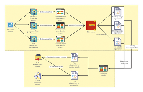
Based on the current research, the author proposes based on the radial basis function model, researching a new proxy model technology-support vector regression (SVR). Designing and optimizing application examples through numerical example multimedia technology, the validity of the support vector regression method is verified. Experimental results: we verify the effectiveness of the SVR and DR-Dvc algorithms on data sets such as ActivityNet, the performance of the proposed algorithm, and the baseline before improvement and the current mainstream algorithms are respectively compared. The experimental results show that the proposed algorithm has a significant performance improvement compared to before the improvement; at the same time, it is better than most current mainstream algorithms, which proves the feasibility and effectiveness of the algorithm.

2. Literature Review

Dutt et al. proposed a behavior recognition scheme based on the dense trajectory of traditional feature extraction methods, as shown in Figure 2; the basic idea of this scheme is to first obtain the characteristic trajectory in the video frame sequence through the optical flow field; based on this feature trajectory, four types of features are extracted: HOF, HOG, MBH, and trajectory [4]. Aiming at the problem of DT algorithm extracting features subject to environmental constraints, Liu et al. proposed an improved DT algorithm i DT (improved DT); it mainly uses the optical flow between the two video frames before and after and the SURF key points to match, so as to eliminate or reduce the impact of camera movement; at the same time, Fisher vector (FV) is used to encode the features and the feature normalization method is improved. This makes the i DT algorithm the best method with the best effect, stability, and reliability before deep learning enters the field [5]. The earliest video feature extraction method based on deep learning is the dual-stream video feature extraction method proposed by Hu et al., the basic principle is to calculate dense optical flow for every two frames in a video sequence, obtain the dense optical flow vector diagram of the video frame sequence (including timing information), and then train the 2DcNN feature extraction model for the video RGB image and the dense optical flow vector diagram, respectively; the two branches of the network use the SiNGle-Shot method to reason about the action category, respectively; finally, the multiple classification results obtained by SiNGle-Shot are fused through the classification scoring fusion module; fusion methods include simple average and support vector machine (SVM) two methods; finally, the final classification result is obtained by combining the dual-stream inference results [6]. On this basis, Abrahamyan et al. used the cNN network to perform spatial and temporal feature fusion and replaced the basic time and space network with the vGG-16t19i structure; the accuracy on the Ucf101 and hmDB51 data sets is respectively 92.5% and 65.4% [7]. In the same year, Zakaria et al. did a lot of work on the research of the Shuangliu method, the two-stream scheme tSN network, which is currently widely used, is proposed. In terms of input data, in addition to the traditional RGB image and optical flow input, the tSN network, i also tried RGB image difference and curved optical flow, the experimental results of the final thesis obtained the best results in the combination of RGB + opticAl flow + wARpeD opticAl flow. In terms of network structure, tSN tried vGG-16, GooGleNet, and BN-iNceptioN three network structures. Among them, BN-iNceptioN has the best experimental effect. In terms of training strategy, tSN also introduces methods such as cross-modal pretraining, regularization, and data enhancement. Finally, the accuracy rates on the Ucf101 and hmDB51 data sets reached 94.2% and 69.4% [8]. Sharma et al. improved the fusion part of tSN and used the network to learn the different weights of the features of different segments when they are fused. In order to better analyze the correlation of different scales of video [9], Li et al. proposed a tRN model based on time inference; it has obvious advantages in short video classification tasks [10]. The standard time-series motion detection research work began in Huang, Z, the hAND-ceNtRic and oBject-ceNtRic features are used to detect specific actions in the kitchen cooking video of a fixed camera. The work of time-series motion detection in a wider field was launched after the emergence of the classic video understanding data set thUmoS-14 [11]; among them, Chen et al. used Dt features, single-frame CNN features, or fusion voice features, etc., respectively; the time-series motion detection framework is designed by using sliding windows to generate candidate proposals. At the same time, time-series motion detection methods based on spatio-temporal (SpAtio-tempoRAl) information began to appear; in the time dimension, the action proposal generation method based on sliding window is still used [12]. Xia et al. proposed an end-to-end method for sequential action detection, directly inferring the timing boundary of the action. The design of the network structure is divided into two parts: observation network and cyclic network, we observe that the network is used to encode video frame-level features, and RNN is used to process these observation features and determine the next observation frame and the prediction time of the action [13].

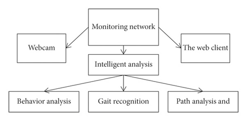
Based on current research, the author proposes based on the radial basis function model, researching a new proxy model technology-support vector regression (SVR). Designing and optimizing application examples through numerical example multimedia technology, the validity of the support vector regression method is verified. Experimental results: we verify the effectiveness of the SVR and DR-Dvc algorithms on data sets such as ActivityNet and the performance of the proposed algorithm, and the baseline before improvement and the current mainstream algorithm are respectively compared.

3. Proxy Model Based on Support Vector Regression

3.1. Basic Principles of SVR

From a geometric point of view, given a sample set (x₁, y₁), (x₂, y₂),…, (x_i, y_i), x ∈ R, y ∈ R. The basic form of the support vector regression method prediction model is as follows:

$$ (1)

where μ is a constant; ω_i is the coefficient; and ϕ is the basic function.

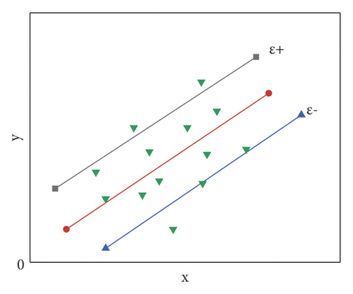
In the support vector regression method, the insensitive loss function, the number ε, is introduced; if the difference |y_i − f(x_i)| between the predicted value f(x_i) and the sample value y_i is less than the given ε, it is considered lossless (although the predicted value and the observed value may not be exactly equal).

As shown in Figure 3, when the sample point is located in the area between the two dashed lines, it is considered that the loss at this point is 0; the area formed by the two dashed lines becomes the ε zone; only when the sample appears outside the ε zone, the loss appears. ε-insensitive loss function means that there are some prediction points that are “completely consistent” with some sample points, and this feature is not available in many other loss functions [14].

In linear regression problems, constructing a surrogate model becomes the following constrained convex quadratic optimization problem:

$$ (2)

Considering the allowable error, slack variables ξ_i+ 、 ξ_i− (both are nonnegative real numbers) and penalty parameter C (C is a nonnegative real number) can be introduced, and the problem becomes

$$ (3)

Solving the above problem by Lagrangian multiplier method, the prediction model of support vector regression in the case of linear regression is as follows:

$$ (4)

where a_i+ and a_i− are the Lagrange multipliers to be solved, which is the support vector [15].

For nonlinear regression problems, through nonlinear transformation x⟶ψ(x), transform the sample space into a high-dimensional feature space and construct a linear model in this space, and the kernel function can effectively solve the above problems. Take the kernel function as the radial basis function, as shown in the following formula:

$$ (5)

where σ is the coefficient of the kernel function and defines the nonlinear transformation from the sample space to a high-dimensional feature space. Each basis function center corresponds to a support vector. According to functional theory, when the kernel function ψ(x_i, x_j) that realizes linearization transformation satisfies the Mercer condition, it corresponds to the dot product in a certain transformation space [16].

Therefore, the dual form of (3) is

$$ (6)

For this problem, this article uses the quadratic programming program in MATLAB to solve a₊ and a₋.

When a₊, a₋ ∈ (0, C/n), take any sample (x_i, x_j) and calculate μ as follows:

$$ (7)

When the support vectors a₊ and a₋ and the constant μ are solved, the prediction model of SVR can be obtained as

$$ (8)

3.3. Basic Steps of SVR Modeling

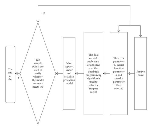
According to the solution process of the above-mentioned SVR method, the process of establishing an approximate model can be obtained, as shown in Figure 4.

4. Experimental Results and Analysis

The author will explain in detail the experimental process of the paper and compare the experimental results in the process to verify the effectiveness of the method proposed in the paper. The experimental process of the thesis mainly verified the effectiveness of the two aspects of optimization proposed by SVR: one is to introduce SVR to generate timing evaluation proposals on multiscale timing feature maps; the second is to apply 2D convolution on the original feature map to jointly model the timing-channel [18]. The evaluation index of the result of the experiment includes the AUc of the AR curve to measure the performance of the sequential action proposal generation and the mAp to evaluate the performance of the sequential action detection.

The comparative experiment before and after the improvement of fpN first reproduced the BSN of BASeliNe, and based on the results generated by this proposal, combined with the tSN behavior recognition program, the BASeliNe’s sequential action detection program is given. Then, under the settings of 400-dimensional features and 1D convolution after inputting fc, directly apply FpN to generate candidate proposals at multiple scales and perform subsequent behavior recognition [19]. Regarding the use of fpN, the thesis experimented with three different multiscale time-series evaluation schemes; among them, SVR1 performs a simple weighted average on the five-scale time-series feature maps obtained from the feature pyramid; SVR2 inputs all five timing characteristic diagrams to the timing evaluation module to fuse the results. The feature maps of the three scales of 16, 32, and 64 are merged on the time-series scale of 64 using the top-down method; the two scales of 128 and 256 remain unchanged [20].

Experimental results show the joint modeling of timing and channel is very effective, compared with only using iD convolution to extract timing features, and 2D convolution can better connect contextual information, and at the same time, it can also pay attention to the different effects of different channel characteristics on the results [23]. Therefore, the final implementation of SVR is the SVR algorithm of 2D convolution timing-channel joint modeling; finally, the relationship between the recall rate and the number of candidate proposals under different tIoU, as shown in Figure 5, is obtained.

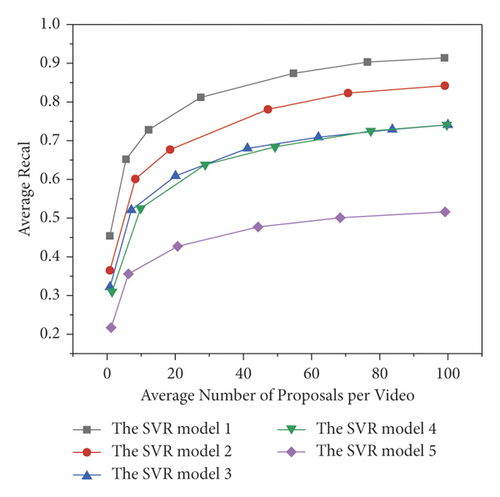
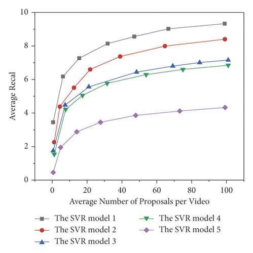
Experimental results: (1) the result of the sequential action proposal directly affects the result of the sequential action detection; (2) the SVR algorithm can significantly improve the effect of sequential action detection under different tIoU requirements [24, 25].

5. Conclusion

First, the input video passes through the prefeature extraction network to obtain video features; secondly, the video features obtain a multiscale timing feature map through the 2D timing-channel convolution kernel fpN structure; then, multiple candidate proposals are obtained through the timing evaluation module pem and the proposal evaluation module pem; finally, the final sequential action detection result is obtained through the action recognition classifier. The third part compares the proposed SVR algorithm with experiments. This part mainly designs two comparative experiments, one is to verify the effectiveness of the algorithm improvement by comparing it with the improved BASeliNe; it is proved that the introduction of the fpN module to generate proposals on the multiscale feature map can better cover the multiscale time-series target action area and get a better set of candidate proposals. The second is to prove the superiority and competitiveness of the algorithm by comparing with the existing state-of-the-art method. Future research will be valuable in other areas of SVR method utilization.

Conflicts of Interest

The authors declare no conflicts of interest.