Understanding the protein-RNA interaction mechanism can help us to further explore various biological processes. The experimental techniques still have some limitations, such as the high cost of economy and time. Predicting protein-RNA-binding sites by using computational methods is an excellent research tool. Here, we developed a universal method for predicting protein-specific RNA-binding sites, so one general model for a given protein was constructed on a fixed dataset by fusing the data of different experimental techniques. At the same time, information theory was employed to characterize the sequence conservation of RNA-binding segments. Conversation difference profiles between binding and nonbinding segments were constructed by information entropy (IE), which indicates a significant difference. Finally, the 19 proteins-specific models based on random forest (RF) were built based on IE encoding. The performance on the independent datasets demonstrates that our method can obtain competitive results when compared with the current best prediction model.

1. Introduction

RNA-binding proteins (RBPs) play an important role in gene expression and regulation since they are highly involved in various biological processes such as mRNA stability [1], stress responses [2], and gene regulation at the transcriptional and posttranscriptional levels [3]. Understanding RNA-protein interactions can lead to further study on the mechanisms underlying these biological processes. Accurate identification of RNA-protein binding sites is very useful for studying these biological processes. In recent years, many high-throughput experimental methods are useful for studying these biological processes. In recent years, many high-throughput experimental methods, such as PAR-CLIP [4], have been developed which can accurately determine the binding sites of RNA-protein interactions at the experimental level. However, these experimental methods are time-consuming and cost-effective. It is necessary to develop computational methods to predict the binding sites between RNAs and proteins.

At present, several researchers have developed computational methods for predicting RNA-protein binding sites. RNA context is a method with sequence and accessibility information to predict binding motifs [5], and Maticzka et al. present GraphProt to predict binding preferences by using RNA sequence and secondary structural contexts [6]. Zhang et al. integrate RNA sequence, secondary structural contexts, and RNA tertiary structural information by using a deep learning framework for modeling structural binding preferences and predicting binding sites of RBPs [7]. Strazar et al. develop an integrative orthogonality-regularized nonnegative matrix factorization (iONMF) to predict RBP interaction sites on RNAs [8]. In iONMF, the features of protein-RNA interactions are the positions of RNA structure and sequence motifs, RBP cobinding, and gene region types. Pan et al. have given iDeep, iDeepS, and iDeepE to predict RNA-protein binding sites from RNA sequences [9]. iDeep developed a novel hybrid convolutional neural network and deep belief network with RNA sequence, secondary structure, clip-cobinding, region type, and motif features to predict the RBP interaction sites and motifs on RNAs. iDeepS can identify the binding sequence and structure motifs from RNA sequences at the same time by using convolutional neural networks and a bidirectional long short-term memory network only with RNA sequence and predicted secondary structure. iDeepE improves the network structure to predict RNA-protein binding sites and motifs by combining local and global deep convolutional neural networks.

The above research has achieved satisfactory prediction results, and some of them obtain the high area under curve (AUC) values in most datasets, such as iDeepS. However, there are still limitations deserving improvement in previous studies, including different experimental datasets and the selection of features.

Since different experimental methods for the same protein are usually different, previous prediction methods are all based on different datasets from different experimental techniques, so multiple different models are usually constructed for a given protein, such as the protein ELAVL1 which has two datasets with different protocols of PAR-CLIP and CLIP-seq [10, 11]. We know that each protein has a definite RNA-binding motif, but there may be some errors that make the RBPs undetectable during the experiment. Different protocols can make up for the loss caused by experimental errors, so different experimental datasets for a given protein could be merged as one general dataset to build a protein-specific model which is universal to different experimental techniques. In addition, the current accuracy of the predicted secondary structures is relatively low, so the reported performance may be of some discount for the existing methods based on the predicted secondary structures.

In our study, we developed a simpler and universal model for predicting RNA-protein binding sites for different proteins only based on RNA sequence information. Firstly, for 19 proteins, 19 general protein-specific datasets were achieved by fusing different experimental data. Then, only based on the sequence information, k-mer-based features and IE profiles were respectively used to represent the binding segments. Finally, the RF model based on IE profiles was proved to be with the best performance, compared with 3, 4, and 5-mer features. The final model yields satisfactory results with an average AUC of 0.849 for the 19 proteins. In addition, the model that uses single RNA secondary structures was also built, but it gives the lowest prediction accuracy. Overall, our method only based on sequence conservation information by IE can obtain competitive results when compared with the current best prediction model.

2. Materials and Methods

2.1. Dataset

We downloaded the datasets from iDeepS [12] which is available at https://github.com/xypan1232/iDeepS. iDeepS collected the data from iONMF [8], and it contains 31 CLIP-seq datasets with 19 binding proteins. Original CLIP-seq data are from servers iCount (http://icount.biolab.si) and DoRiNA [13]. In the iDeepS datasets, protein-RNA-binding sites are positive samples. Fifty bases were selected from each side of the binding site by sliding window to form a sequence with a length of 101. Genes that had never been identified as interacting sites in 31 experiments were used as negative samples.

In our work, in order to construct the protein-specific and experiment-universal model, we merged 31 CLIP-seq datasets into 19 general datasets for 19 different proteins. Here, due to the different structures, Ago2-MNase and Ago2, as well as ELAVL1-MNase and ELAVL1, are deemed as different proteins from each other [14]. Finally, we separated each dataset into training and testing one according to the ratio of 5 : 1. The detailed information about the 19 datasets is shown in Table 1.

Table 1. The prediction performance of the models constructed with a single information entropy feather across 31 original experiment datasets.

Training groups	Protein	SE	SP	ACC	MCC	AUC_train	AUC_test
A	1 Ago/EIF	0.500	0.504	0.502	0.004	0.605	0.583
	3 Ago2-1	0.523	0.444	0.490	−0.032		0.623
	4 Ago2-2	0.515	0.548	0.528	0.062		0.656
	5 Ago2	0.473	0.508	0.489	−0.019		0.554
B	6 eIF4AIII-1	0.745	0.845	0.795	0.593	0.851	0.858
B	7 eIF4AIII-2	0.780	0.805	0.793	0.585		0.873
C	8 ELAVL1-1	0.860	0.118	0.501	−0.033	0.750	0.715
	10 ELAVL1A	0.763	0.119	0.460	−0.153		0.626
	11 ELAVL1-2	0.869	0.090	0.501	−0.065		0.703
D	12 ESWR1	0.870	0.735	0.803	0.611	0.858	0.896
E	13 FUS	0.885	0.855	0.870	0.740	0.916	0.914
E	14 Mut FUS	0.890	0.840	0.865	0.731		0.912
F	15 IGFBP1-3	0.690	0.675	0.683	0.365	0.628	0.771
G	16 hnRNPC-1	0.595	0.840	0.718	0.449	0.947	0.830
G	17 hnRNPC-2	0.685	0.835	0.760	0.526		0.844
H	18 hnRNPL-1	0.680	0.750	0.715	0.431	0.754	0.810
	19 hnRNPL-2	0.740	0.730	0.735	0.470		0.805
	20 hnRNPL-like	0.625	0.710	0.668	0.336		0.732
I	21 MOV10	0.960	0.535	0.748	0.547	0.776	0.835
J	22 Nsun2	0.685	0.745	0.715	0.431	0.832	0.796
K	23 PUM2	0.920	0.795	0.858	0.721	0.887	0.915
L	24 QKI	0.840	0.890	0.865	0.731	0.920	0.937
M	25 SRSF1	0.705	0.795	0.750	0.502	0.785	0.848
N	26 TAF15	0.885	0.855	0.870	0.740	0.906	0.930
O	27 TDP-43	0.815	0.845	0.830	0.660	0.819	0.889
P	28 TIA1	0.760	0.875	0.818	0.639	0.999	0.900
P	29 TIAL1	0.645	0.840	0.743	0.494		0.842
Q	30 U2AF2	0.780	0.855	0.818	0.637	0.901	0.903
Q	31 U2AF2 (KD)	0.700	0.865	0.783	0.573		0.874
R	2 Ago2-MNase	0.239	0.659	0.451	−0.113	0.605	0.405
S	9 ELAVL1-MNase	0.719	0.245	0.491	−0.040	0.605	0.499

2.2. Methods

2.2.1. Feature Extraction

Here, we tried to represent protein binding RNAs from RNA primary sequences by IE profiles and K-mer features. Besides, since RNA secondary structures have been used and demonstrated to be useful for representing binding segments by previous reports [15], they were also extracted to be compared with features from sequence information.

(1) Information Entropy. Information entropy (IE) was proposed by Shannon [16] and has been deemed as one of the simplest and most common measures of conservation at a site on protein sequences in the field of bioinformatics [17]. IE describes the occurrence probability of discrete random events, and it also reflects the evolutionary conservatism of each location in the sequence. It has been successfully used in our previous research works of Shi et al. [18] and Wang et al. [19]. Shi et al. used IE to distinguish the difference between methylated and nonmethylated peptide segments, and Wang et al. used it to classify Type IV secreted effectors from the negative sample based on the N-terminal 100 residues.

In our work, IE is used to measure evolutionary conservation differences between binding and nonbinding sites of RNA sequences. The information content of each nucleic base at each position can be calculated as the input features to predict protein-RNA interaction binding sites.

(2) K-mer. K-mer is a common genomic feature in bioinformatics, and it has been widely used to identify some regions in biological DNA or protein molecules. Zhang et al. use K-mer to predict piRNA [20], and Cao et al. make use of K-mer to predict subcellular localization of lncRNA [21]. To characterize protein binding RNA sequences, we used all the 3–5 nt strings, including 3mer strings, 4mer strings, and 5mer strings.

(3) RNA Secondary Structure. RNA secondary structure refers to the planar structure formed by various components, such as single-stranded region structure, stem-ring structure, and double-stranded structure, which are composed of complementary base pairs in an RNA molecule and self-folding through these structures. RNA secondary structure is a kind of reversal formed by RNA molecules under natural conditions.

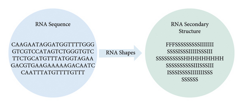
RNA secondary structures are widely used in protein-RNA-binding site prediction, such as iONMF [8] and iDeepS [22]. RNAshapes is a tool for predicting the secondary structure of RNA [23]. We used RNAshapes to obtain RNA secondary structure annotations by referring to Fukunaga et al. [24]. In this way, we can obtain the secondary structure of each position in the sequence (Figure 1). Six types of secondary structures were considered, including stems (S), multiloops (M), hairpins (H), internal loops (I), dangling end (T), and dangling start (F).

Details are in the caption following the image — **Figure 1**
Open in figure viewer PowerPoint

Conversion diagram of RNA secondary structure.

2.2.2. Random Forests

The random forests (RFs) algorithm is an integrated classification model [25]. Its construction process is mainly composed of three aspects: the generation of a training set, the construction of a decision tree, and the generation of the algorithm. First, we need to generate training sets from the original data by sampling. Through the bagging algorithm, N samples are extracted from the original data set. Each sample will produce a decision tree, and the generated decision tree does not need pruning, thus establishing N decision trees to form forests.

At present, the RF algorithm is one of the most popular machine learning algorithms, and it has been widely used to solve biological classification [26–30].

The RF model we used in this study was implemented by a random forest package in the R language.

2.2.3. Evaluation Indicators

We used five effective performance evaluation indicators to evaluate the predictive ability of the model, namely area under curve (AUC), sensitivity (SE), specificity (SP), accuracy (ACC), and Matthew's correlation coefficient (MCC), respectively. AUC represents the area under the receiver operating characteristic (ROC) curve. When drawing the ROC curve, the true positive is taken as ordinate, and the false positive is taken as abscissa. The closer the AUC is to 1, the better the prediction will be these metrics are commonly defined as follows:

(1)

where TP, FP, TN, and FN are true positive, false positive, true negative, and false negative, respectively.

3. Results and Discussion

3.1. Difference Analysis between Positive and Negative Samples

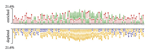
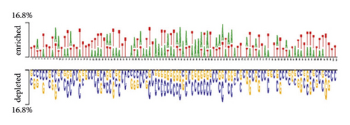
The distribution of nucleic bases is the basic information for an RNA sequence. With the segment length of 101 bases, we plotted two sample logos [15, 31] of 19 protein training sets to show the difference in base composition between positive and negative samples in each dataset. Here, we select two of them as examples. We can find that the positive and negative samples of the same protein have obvious differences in base compositions. For each segment, the 51st base in the positive sample sequence is the protein-RNA interaction site. According to the literature [32], the binding motif of protein-RNA interaction is usually 6–8 bases. From Figure 2(a), we can find that the (Figure 2) base locations of 48–54 in positive samples are obviously enriched with A and T. Negative samples were not enriched with A and T. Similarly, for the MOV10 data set, we can find that the 48–54 base positions of positive samples have obvious C and G enrichment from Figure 2(c). Especially at the 51st position of the positive sample, there was a significant C base enrichment. Negative samples do not have the above observations. Thus, the difference in base composition between positive and negative samples is significant.

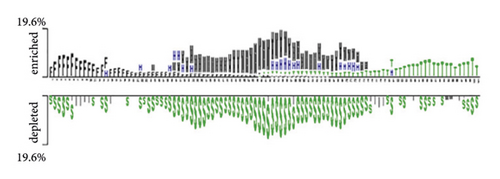
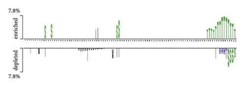
We also plotted the two sample logos of the secondary structure of 19 protein training sets and showed the difference in the secondary structure of positive and negative samples for each data set. When protein and RNA interact, they both have unique space structures [33]. Therefore, the secondary structure of positive and negative samples will be different. It is also proved by our two sample logos. In Figure 2(b), we can find that the 48–54 positions in the positive samples of QKI datasets are usually multiloop (M) and hairpin (H). In the secondary structure of negative samples, we find that there are more stem (S) structures. In Figure 2(d), the positive sample of the MOV10 dataset is stem (S) structures at 48–54 positions. Negative samples did not show many stem (S) structures. We can also find that the positive and negative samples have obvious secondary structure differences by using two sample logos.

Then, we calculated the information entropy of 19 datasets. Information entropy can characterize the evolutionary conservation of each position in a sequence. We selected two training datasets of PUM2 and TIA1 to show the results of IE difference between positive and negative samples in Figure 3. From Figure 3, we can find that the IE values of positive and negative samples have obvious differences. We know that the lower the IE value of a given position is, the more conservative this position is. In general, we can easily see that all bases in the positive dataset are more conservative than those in the negative dataset. Moreover, there are significant conservation differences between positive and negative samples at the location of the 51st base and its adjacent bases, as marked by the red ovals in Figure 3.

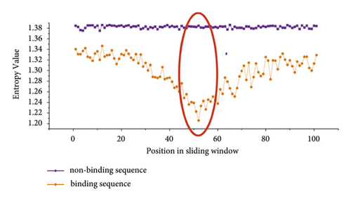
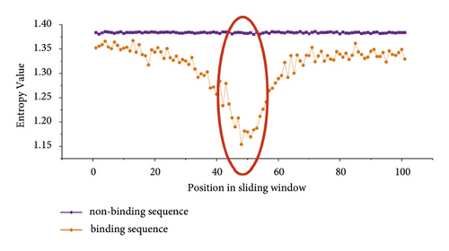
The large difference in sequence conservativeness between binding and nonbinding sequences means that IE will be an important feature for predicting potential protein-RNA interaction sites.

3.2. Results on the Original 31 Datasets and the Combined 19 Datasets

According to the definition of IE and IG, we calculated the IG value of each position in the sequence. The IG value can quantitatively reflect the evolutionary conservation of each site in the sequence. We can find that the evolutionary conservatism of positive and negative samples is obviously different. Firstly, we use a single IG as the feature to construct the classifying model. Figure 4 shows the AUC of 31 original test sets. The average AUC value of test datasets is 0.86, which indicates that IE is generally effective for predicting binding sites of protein-RNA interactions.

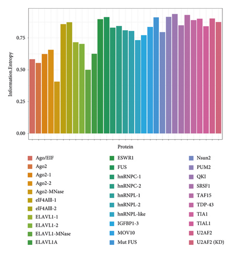
In order to get a more general model, we merged the datasets from different experiments for the same protein, so 19 protein-specific datasets were achieved. According to 19 proteins, the protein-specific model for each protein was constructed on each protein-specific dataset. Figure 5 shows the AUCs of the combined test datasets, and Table 2 lists the detailed information. We can find that IE-based models also yield good prediction performance with an average AUC of 0.807. Moreover, 12 of 19 models give the AUC values higher than 0.8. The results of test datasets indicate that the general prediction model for each protein is valid, and it is a feasible way to develop the protein-specific model for the data from different experiments.

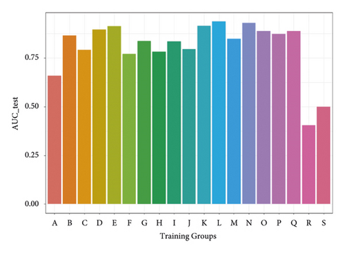
Table 2. The prediction performance of the models is constructed with a single information entropy feather across 19 merged experiment datasets.

Training groups	SE	SP	ACC	MCC	AUC_train	AUC_test
A	0.635	0.607	0.621	0.217	0.639	0.659
B	0.765	0.820	0.793	0.465	0.847	0.865
C	0.734	0.708	0.721	0.368	0.777	0.792
D	0.870	0.735	0.803	0.482	0.858	0.896
E	0.885	0.848	0.866	0.557	0.916	0.914
F	0.690	0.675	0.683	0.312	0.628	0.771
G	0.640	0.838	0.739	0.400	0.947	0.837
H	0.682	0.730	0.706	0.347	0.754	0.783
I	0.960	0.535	0.748	0.447	0.776	0.835
J	0.685	0.745	0.715	0.360	0.832	0.796
K	0.920	0.795	0.858	0.550	0.887	0.915
L	0.840	0.890	0.865	0.556	0.920	0.937
M	0.705	0.795	0.750	0.410	0.785	0.848
N	0.885	0.855	0.870	0.561	0.906	0.930
O	0.815	0.845	0.830	0.513	0.819	0.889
P	0.700	0.865	0.783	0.458	0.999	0.874
Q	0.743	0.860	0.801	0.479	0.901	0.888
R	0.239	0.659	0.451	−0.113	0.605	0.405
S	0.719	0.245	0.491	−0.040	0.605	0.499

Secondly, six protein training sets were selected from 19 proteins according to the results of the model constructed with a single information entropy feather. Table 3 shows the AUC comparison of three models based on the features of K = 3, 4, and 5, respectively. The result of 4-mer is similar to that of 5-mer and better than that of 3-mer. When K = 5, the feature dimension is 1028, so there are many positions in 1028 features with a result of 0. In order to reduce the noise of the model, we give up 5-mer as a feature. Finally, we chose K = 4.

Table 3. AUCs of 6 selected proteins with a single K-mer.

Protein	AUC of 3-mer	AUC of 4-mer	AUC of 5-mer
QKI	0.9	0.899	0.919
U2AF2	0.871	0.8871	0.886
SRSF1	0.853	0.856	0.867
Mut FUS	0.829	0.836	0.841
Nsun2	0.76	0.763	0.767
IGFBP1-3	0.657	0.675	0.686

Previous research has selected secondary structures as a feature to predict protein-RNA interaction binding sites [7]. We also tried to introduce the secondary structure into our prediction model. Table 4 is the test sets AUC of the original 31 datasets using the secondary structure separately. However, we find that the contribution of a single secondary structure to the model is very small. The average AUC is only 0.55. There are specific secondary structures when proteins interact with RNA. But the RNA secondary structure used in current research is not the real secondary structure. They are derived from predictive tools such as RNAshapes [23] and RNAfold [34]. So, it will provide some wrong information to the model. Because the secondary structure cannot provide a positive impact on the prediction performance of the model, we do not choose to add the secondary structure to the final prediction model.

Table 4. The prediction performance of the models is constructed with a single secondary structure feather across 31 original experiment datasets.

Training groups	Protein	SE	SP	ACC	MCC	AUC train	AUC test
A	1 Ago/EIF	0.505	0.500	0.503	0.005	0.537	0.513
	3 Ago2-1	0.420	0.555	0.488	−0.025		0.509
	4 Ago2-2	0.440	0.580	0.510	0.020		0.510
	5 Ago2	0.530	0.420	0.475	−0.050		0.464
B	6 eIF4AIII-1	0.035	0.965	0.500	0.000	0.560	0.547
B	7 eIF4AIII-2	0.350	0.745	0.548	0.103		0.600
C	8 ELAVL1-1	0.895	0.090	0.493	−0.025	0.632	0.498
	10 ELAVL1A	0.635	0.410	0.523	0.046		0.533
	11 ELAVL1-2	0.620	0.620	0.620	0.240		0.662
D	12 ESWR1	0.460	0.640	0.550	0.102	0.582	0.555
E	13 FUS	0.565	0.550	0.558	0.115	0.630	0.578
E	14 Mut FUS	0.565	0.710	0.638	0.278		0.642
F	15 IGFBP1-3	0.565	0.710	0.638	0.278	0.523	0.642
G	16 hnRNPC-1	0.500	0.745	0.623	0.253	0.679	0.661
G	17 hnRNPC-2	0.335	0.915	0.625	0.307		0.670
H	18 hnRNPL-1	0.540	0.500	0.520	0.040	0.573	0.551
	19 hnRNPL-2	0.505	0.600	0.553	0.105		0.564
	20 hnRNPL-like	0.465	0.510	0.488	−0.025		0.470
I	21 MOV10	0.440	0.580	0.510	0.020	0.521	0.520
J	22 Nsun2	0.615	0.530	0.573	0.146	0.610	0.595
K	23 PUM2	0.600	0.590	0.595	0.190	0.565	0.625
L	24 QKI	0.600	0.590	0.595	0.190	0.724	0.625
M	25 SRSF1	0.085	0.910	0.498	−0.009	0.522	0.464
N	26 TAF15	0.580	0.625	0.603	0.205	0.609	0.618
O	27 TDP-43	0.580	0.625	0.603	0.205	0.553	0.618
P	28 TIA1	0.155	0.955	0.555	0.183	1.000	0.636
P	29 TIAL1	0.120	0.950	0.535	0.126		0.567
Q	30 U2AF2	0.120	0.950	0.535	0.126	0.602	0.567
Q	31 U2AF2 (KD)	0.330	0.705	0.518	0.038		0.548
R	2 Ago2-MNase	0.545	0.470	0.508	0.015	0.499	0.516
S	9 ELAVL1-MNase	0.485	0.550	0.518	0.035	0.519	0.506

3.3. Comparison of Our Work and Other’s works

Finally, we construct a hybrid model to predict protein-RNA interaction binding sites by combining IE with 4-mer. Then, the two models constructed by us with IE and IE + 4-mer were compared with the reported tool of iDeepS [12]. Table 5 shows the comparisons among the three models. On average, the hybrid model based on IE + 4-mer is superior to the model only with IE. For most datasets, the prediction performance of the hybrid model is almost equal to that of iDeepS. The average AUC of our hybrid model is 0.849, and that of iDeepS is 0.863. However, iDeepS is a tool based on sequence and secondary structure information. Our hybrid model is only sequence information. So, it is more concise and practical.

Table 5. The comparison results among the model of single information entropy, the model of single information entropy with 4-mer, and iDeepS.

Protein	Information entropy	Information entropy + 4-mer	iDeepS
1 Ago/EIF	0.583	0.708	0.773
3 Ago2-1	0.623	0.832	0.865
4 Ago2-2	0.656	0.839	0.868
5 Ago2	0.554	0.592	0.634
6 eIF4AIII-1	0.858	0.932	0.950
7 eIF4AIII-2	0.873	0.934	0.953
8 ELAVL1-1	0.715	0.921	0.932
10 ELAVL1A	0.626	0.875	0.893
11 ELAVL1-2	0.703	0.907	0.919
12 ESWR1	0.896	0.904	0.917
13 FUS	0.914	0.936	0.934
14 Mut FUS	0.912	0.920	0.958
15 IGFBP1-3	0.771	0.709	0.717
16 hnRNPC-1	0.830	0.929	0.960
17 hnRNPC-2	0.844	0.966	0.975
18 hnRNPL-1	0.810	0.827	0.756
19 hnRNPL-2	0.805	0.802	0.769
20 hnRNPL-like	0.732	0.746	0.711
21 MOV10	0.835	0.839	0.813
22 Nsun2	0.796	0.811	0.835
23 PUM2	0.915	0.963	0.962
24 QKI	0.937	0.945	0.966
25 SRSF1	0.848	0.873	0.887
26 TAF15	0.930	0.934	0.964
27 TDP-43	0.889	0.913	0.930
28 TIA1	0.900	0.911	0.930
29 TIAL1	0.842	0.856	0.893
30 U2AF2	0.903	0.921	0.953
31 U2AF2 (KD)	0.874	0.891	0.931
2 Ago2-MNase	0.405	0.615	0.591
9 ELAVL1-MNase	0.499	0.566	0.613

The prediction performance of the models constructed with information entropy and 4-mer feather across 31 original experiment datasets can be seen in Table 6. The detailed comparison results are shown in Table 5.

Table 6. The prediction performance of the models is constructed with information entropy and 4-mer feather across 31 original experiment datasets.

Training groups	Protein	SE	SP	ACC	MCC	AUC_train	AUC_test
A	1 Ago/EIF	0.530	0.730	0.630	0.265	0.750	0.708
	3 Ago2-1	0.815	0.680	0.748	0.500	0.750	0.832
	4 Ago2-2	0.805	0.700	0.753	0.508	0.750	0.839
	5 Ago2	0.365	0.720	0.543	0.091	0.750	0.592
B	6 eIF4AIII-1	0.810	0.875	0.843	0.686	0.924	0.932
B	7 eIF4AIII-2	0.870	0.835	0.853	0.705	0.924	0.934
C	8 ELAVL1-1	0.925	0.755	0.840	0.690	0.897	0.921
	10 ELAVL1A	0.850	0.755	0.803	0.608	0.897	0.875
	11 ELAVL1-2	0.890	0.720	0.805	0.619	0.897	0.907
D	12 ESWR1	0.850	0.800	0.825	0.651	0.845	0.904
E	13 FUS	0.870	0.875	0.873	0.745	0.895	0.936
E	14 Mut FUS	0.830	0.885	0.858	0.716	0.895	0.920
F	15 IGFBP1-3	0.690	0.560	0.625	0.252	0.695	0.709
G	16 hnRNPC-1	0.865	0.850	0.858	0.715	0.952	0.929
G	17 hnRNPC-2	0.960	0.870	0.915	0.833	0.952	0.966
H	18 hnRNPL-1	0.775	0.725	0.750	0.501	0.765	0.827
	19 hnRNPL-2	0.780	0.715	0.748	0.496	0.765	0.802
	20 hnRNPL-like	0.645	0.735	0.690	0.382	0.765	0.746
I	21 MOV10	0.875	0.655	0.765	0.543	0.793	0.839
J	22 Nsun2	0.725	0.735	0.730	0.460	0.832	0.811
K	23 PUM2	0.920	0.870	0.895	0.791	0.927	0.963
L	24 QKI	0.895	0.855	0.875	0.751	0.941	0.945
M	25 SRSF1	0.785	0.790	0.788	0.575	0.858	0.873
N	26 TAF15	0.870	0.890	0.880	0.760	0.897	0.934
O	27 TDP-43	0.750	0.875	0.813	0.630	0.888	0.913
P	28 TIA1	0.775	0.900	0.838	0.680	0.998	0.911
P	29 TIAL1	0.645	0.875	0.760	0.534	0.998	0.856
Q	30 U2AF2	0.865	0.810	0.838	0.676	0.895	0.921
Q	31 U2AF2 (KD)	0.855	0.760	0.808	0.618	0.895	0.891
R	2 Ago2-MNase	0.545	0.625	0.585	0.171	0.605	0.615
S	9 ELAVL1-MNase	0.280	0.755	0.518	0.040	0.593	0.566

4. Conclusions

In this work, we have developed a simpler and more applied model for predicting protein-RNA interaction binding sites. According to the same binding protein, we merged the original datasets from different experiments, so the model constructed by the merged dataset is more general. We compared the performance of the prediction models with single IE, K-mer, and RNA secondary structures, respectively, and we found that models based on single IE and single 4-mer give satisfactory performance. Then, we constructed a hybrid model based on IE + 4-mer and compared it with the reported tool of iDeepS. We find that our hybrid model gives a competitive performance. However, in this paper, we first develop a general model for a specific protein, and our model is only based on the sequence information, so it is more feasible than other tools based on RNA structures.

Conflicts of Interest

The authors declare that they have no conflicts of interest.

Open Research

Data Availability

The dataset can be accessed upon request.

References

1 Jacobs Anderson J. S. and Parker R., Computational identification of cis-acting elements affecting post-transcriptional control of gene expression in Saccharomyces cerevisiae, Nucleic Acids Research. (2000) 28, no. 7, 1604–1617, https://doi.org/10.1093/nar/28.7.1604.
10.1093/nar/28.7.1604
CAS PubMed Web of Science® Google Scholar
2 Abdelmohsen K., Kuwano Y., Kim H. H., and Gorospe M., Posttranscriptional gene regulation by RNA-binding proteins during oxidative stress: implications for cellular senescence, Bchm. (2008) 389, no. 3, 243–255, https://doi.org/10.1515/bc.2008.022, 2-s2.0-40149096226.
10.1515/BC.2008.022
CAS Google Scholar
3 Noller H. F., RNA structure: reading the ribosome, Science. (2005) 309, no. 5740, 1508–1514, https://doi.org/10.1126/science.1111771, 2-s2.0-24644437810.
10.1126/science.1111771
CAS PubMed Web of Science® Google Scholar
4 Hafner M., Landthaler M., Burger L., Khorshid M., Hausser J., Berninger P., Rothballer A., Ascano Jr. M., Jungkamp A.-C., Munschauer M., Ulrich A., Wardle G. S., Dewell S., Zavolan M., and Tuschl T., Transcriptome-wide identification of RNA-binding protein and microRNA target sites by PAR-CLIP, Cell. 2010a, 141, no. 1, 129–141, https://doi.org/10.1016/j.cell.2010.03.009, 2-s2.0-77950920903.
10.1016/j.cell.2010.03.009
CAS PubMed Web of Science® Google Scholar
5 Kazan H., Ray D., Chan E. T., Hughes T. R., and Morris Q., RNAcontext: a new method for learning the sequence and structure binding preferences of RNA-binding proteins, PLoS Computational Biology. (2010) 6, no. 7, e1000832, https://doi.org/10.1371/journal.pcbi.1000832, 2-s2.0-78049275913.
10.1371/journal.pcbi.1000832
CAS PubMed Web of Science® Google Scholar
6 Maticzka D., Lange S. J., Costa F., and Backofen R., GraphProt: modeling binding preferences of RNA-binding proteins, Genome Biology. (2014) 15, R17–R18, https://doi.org/10.1186/gb-2014-15-1-r17, 2-s2.0-84892636681.
10.1186/gb-2014-15-1-r17
CAS PubMed Web of Science® Google Scholar
7 Zhang S., Zhou J., Hu H., Gong H., Chen L., Cheng C., and Zeng J., A deep learning framework for modeling structural features of RNA-binding protein targets, Nucleic Acids Research. (2016) 44, no. 4, https://doi.org/10.1093/nar/gkv1025, 2-s2.0-84960503750.
10.1093/nar/gkv1025
Web of Science® Google Scholar
8 Stražar M., Žitnik M., Zupan B., Ule J., and Curk T., Orthogonal matrix factorization enables integrative analysis of multiple RNA binding proteins, Bioinformatics. (2016) 32, no. 10, 1527–1535, https://doi.org/10.1093/bioinformatics/btw003, 2-s2.0-84970024013.
10.1093/bioinformatics/btw003
CAS PubMed Web of Science® Google Scholar
9 Pan X. and Shen H.-B., RNA-protein binding motifs mining with a new hybrid deep learning based cross-domain knowledge integration approach, BMC Bioinformatics. (2017) 18, no. 1, https://doi.org/10.1186/s12859-017-1561-8, 2-s2.0-85014099241.
10.1186/s12859-017-1561-8
Web of Science® Google Scholar
10 Hafner M., Landthaler M., Burger L., Khorshid M., Hausser J., Berninger P., Rothballer A., Ascano M., Jungkamp A.-C., Munschauer M., Ulrich A., Wardle G. S., Dewell S., Zavolan M., and Tuschl T., PAR-CliP-a method to identify transcriptome-wide the binding sites of RNA binding proteins, Journal of Visualized Experiments: Journal of Visualized Experiments. 2010b, no. 41, e2034, https://doi.org/10.3791/2034, 2-s2.0-80055101895.
10.3791/2034
PubMed Google Scholar
11 Licatalosi D. D., Mele A., Fak J. J., Ule J., Kayikci M., Chi S. W., Clark T. A., Schweitzer A. C., Blume J. E., Wang X., Darnell J. C., and Darnell R. B., HITS-CLIP yields genome-wide insights into brain alternative RNA processing, Nature. (2008) 456, no. 7221, 464–469, https://doi.org/10.1038/nature07488, 2-s2.0-56549105330.
10.1038/nature07488
CAS PubMed Web of Science® Google Scholar
12 Pan X., Rijnbeek P., Yan J., and Shen H.-B., Prediction of RNA-protein sequence and structure binding preferences using deep convolutional and recurrent neural networks, BMC Genomics. (2018) 19, no. 1, https://doi.org/10.1186/s12864-018-4889-1, 2-s2.0-85049451860.
10.1186/s12864-018-4889-1
Web of Science® Google Scholar
13 Anders G., Mackowiak S. D., Jens M., Maaskola J., Kuntzagk A., Rajewsky N., Landthaler M., and Dieterich C., doRiNA: a database of RNA interactions in post-transcriptional regulation, Nucleic Acids Research. (2012) 40, no. D1, D180–D186, https://doi.org/10.1093/nar/gkr1007, 2-s2.0-84861963461.
10.1093/nar/gkr1007
CAS PubMed Web of Science® Google Scholar
14 Leung A. K. L., Young A. G., Bhutkar A., Zheng G. X., Bosson A. D., Nielsen C. B., and Sharp P. A., Erratum: genome-wide identification of Ago2 binding sites from mouse embryonic stem cells with and without mature microRNAs, Nature Structural & Molecular Biology. (2011) 18, no. 9, https://doi.org/10.1038/nsmb0911-1084a, 2-s2.0-80052471736.
10.1038/nsmb0911-1084a
PubMed Web of Science® Google Scholar
15 Ray D., Kazan H., Cook K. B., Weirauch M. T., Najafabadi H. S., Li X., Gueroussov S., Albu M., Zheng H., Yang A., Na H., Irimia M., Matzat L. H., Dale R. K., Smith S. A., Yarosh C. A., Kelly S. M., Nabet B., Mecenas D., Li W., Laishram R. S., Qiao M., Lipshitz H. D., Piano F., Corbett A. H., Carstens R. P., Frey B. J., Anderson R. A., Lynch K. W., Penalva L. O. F., Lei E. P., Fraser A. G., Blencowe B. J., Morris Q. D., and Hughes T. R., A compendium of RNA-binding motifs for decoding gene regulation, Nature. (2013) 499, no. 7457, 172–177, https://doi.org/10.1038/nature12311, 2-s2.0-84880427394.
10.1038/nature12311
CAS PubMed Web of Science® Google Scholar
16 Núñez J., Cincotta P., and Wachlin F., Information Entropy. Chaos In Gravitational N-Body Systems, 1996, Springer, Berlin, Germany.
Google Scholar
17 Sander C. and Schneider R., Database of homology-derived protein structures and the structural meaning of sequence alignment, Proteins: Structure, Function, and Genetics. (1991) 9, no. 1, 56–68, https://doi.org/10.1002/prot.340090107, 2-s2.0-0026030641.
10.1002/prot.340090107
CAS PubMed Web of Science® Google Scholar
18 Shi Y., Guo Y., Hu Y., and Li M., Position-specific prediction of methylation sites from sequence conservation based on information theory, Scientific Reports. (2015) 5, 12403–12414, https://doi.org/10.1038/srep12403, 2-s2.0-84937867545.
10.1038/srep12403
CAS PubMed Web of Science® Google Scholar
19 Wang Y., Guo Y., Pu X., and Li M., Effective prediction of bacterial type IV secreted effectors by combined features of both C-termini and N-termini, Journal of Computer-Aided Molecular Design. (2017) 31, no. 11, 1029–1038, https://doi.org/10.1007/s10822-017-0080-z, 2-s2.0-85033496628.
10.1007/s10822-017-0080-z
CAS PubMed Web of Science® Google Scholar
20 Zhang Y., Wang X., and Kang L., A k-mer scheme to predict piRNAs and characterize locust piRNAs, Bioinformatics. (2011) 27, no. 6, 771–776, https://doi.org/10.1093/bioinformatics/btr016, 2-s2.0-79952589852.
10.1093/bioinformatics/btr016
CAS PubMed Web of Science® Google Scholar
21 Cao Z., Pan X., Yang Y., Huang Y., and Shen H.-B., The lncLocator: a subcellular localization predictor for long non-coding RNAs based on a stacked ensemble classifier, Bioinformatics. (2018) 34, no. 13, 2185–2194, https://doi.org/10.1093/bioinformatics/bty085, 2-s2.0-85047121403.
10.1093/bioinformatics/bty085
CAS PubMed Web of Science® Google Scholar
22 Pan X. and Shen H.-B., Predicting RNA–protein binding sites and motifs through combining local and global deep convolutional neural networks, Bioinformatics. (2018) 34, no. 20, 3427–3436, https://doi.org/10.1093/bioinformatics/bty364, 2-s2.0-85049489507.
10.1093/bioinformatics/bty364
CAS PubMed Web of Science® Google Scholar
23 Steffen P., Voss B., Rehmsmeier M., Reeder J., and Giegerich R., RNAshapes: an integrated RNA analysis package based on abstract shapes, Bioinformatics. (2006) 22, no. 4, 500–503, https://doi.org/10.1093/bioinformatics/btk010, 2-s2.0-32544440797.
10.1093/bioinformatics/btk010
CAS PubMed Web of Science® Google Scholar
24 Fukunaga T., Ozaki H., Terai G., Asai K., Iwasaki W., and Kiryu H., CapR: revealing structural specificities of RNA-binding protein target recognition using CLIP-seq data, Genome Biology. (2014) 15, no. 1, https://doi.org/10.1186/gb-2014-15-1-r16, 2-s2.0-84892606476.
10.1186/gb-2014-15-1-r16
PubMed Web of Science® Google Scholar
25 Breiman L., Random forests, Machine Learning. (2001) 45, no. 1, 5–32, https://doi.org/10.1023/a:1010933404324, 2-s2.0-0035478854.
10.1023/A:1010933404324
Web of Science® Google Scholar
26 Luo J., Guo Y., Zhong Y., Ma D., Li W., and Li M., A functional feature analysis on diverse protein–protein interactions: application for the prediction of binding affinity, Journal of Computer-Aided Molecular Design. (2014) 28, no. 6, 619–629, https://doi.org/10.1007/s10822-014-9746-y, 2-s2.0-84902766842.
10.1007/s10822-014-9746-y
CAS PubMed Web of Science® Google Scholar
27 Luo J., Li W., Liu Z., Guo Y., Pu X., and Li M., A sequence-based two-level method for the prediction of type I secreted RTX proteins, Analyst. (2015) 140, no. 9, 3048–3056, https://doi.org/10.1039/c5an00311c, 2-s2.0-84928327371.
10.1039/C5AN00311C
CAS PubMed Web of Science® Google Scholar
28 Wang Y., Guo Y., Kuang Q., Pu X., Ji Y., Zhang Z., and Li M., A comparative study of family-specific protein–ligand complex affinity prediction based on random forest approach, Journal of Computer-Aided Molecular Design. (2015) 29, no. 4, 349–360, https://doi.org/10.1007/s10822-014-9827-y, 2-s2.0-84925496993.
10.1007/s10822-014-9827-y
CAS PubMed Web of Science® Google Scholar
29 Qiu H., Guo Y., Yu L., Pu X., and Li M., Predicting protein lysine methylation sites by incorporating single-residue structural features into Chou's pseudo components, Chemometrics and Intelligent Laboratory Systems. (2018) 179, 31–38, https://doi.org/10.1016/j.chemolab.2018.05.007, 2-s2.0-85048321596.
10.1016/j.chemolab.2018.05.007
CAS Web of Science® Google Scholar
30 Hu W., Qin L., Li M., Pu X., and Guo Y., Individually double minimum-distance definition of protein–RNA binding residues and application to structure-based prediction, Journal of Computer-Aided Molecular Design. (2018) 32, no. 12, 1363–1373, https://doi.org/10.1007/s10822-018-0177-z, 2-s2.0-85057310352.
10.1007/s10822-018-0177-z
CAS PubMed Web of Science® Google Scholar
31 Schneider T. D. and Stephens R. M., Sequence logos: a new way to display consensus sequences, Nucleic Acids Research. (1990) 18, no. 20, 6097–6100, https://doi.org/10.1093/nar/18.20.6097, 2-s2.0-0025008168.
10.1093/nar/18.20.6097
CAS PubMed Web of Science® Google Scholar
32 Crooks G. E., Hon G., Chandonia J.-M., and Brenner S. E., WebLogo: a sequence logo generator: figure 1, Genome Research. (2004) 14, no. 6, 1188–1190, https://doi.org/10.1101/gr.849004, 2-s2.0-2142738304.
10.1101/gr.849004
CAS PubMed Web of Science® Google Scholar
33 Li X., Kazan H., Lipshitz H. D., and Morris Q. D., Finding the target sites of RNA-binding proteins, Wiley Interdisciplinary Reviews: RNA. (2014) 5, 111–130, https://doi.org/10.1002/wrna.1201, 2-s2.0-84890294599.
10.1002/wrna.1201
CAS PubMed Web of Science® Google Scholar
34 Hofacker I. L., Vienna RNA secondary structure server, Nucleic Acids Research. (2003) 31, no. 13, 3429–3431, https://doi.org/10.1093/nar/gkg599, 2-s2.0-0043123153.
10.1093/nar/gkg599
CAS PubMed Web of Science® Google Scholar

All articles

Protein-Specific Prediction of RNA-Binding Sites Based on Information Entropy

Abstract

1. Introduction