This paper takes the data of a university graduate as the research object. By consulting various literatures and literature analyses, we can understand the impact of students’ academic performance, English level, and other activities on students’ employment development and select data on this basis. The collected data is cleaned, integrated, and transformed to form a standard data set. The factors affecting graduates’ employment are complex and diverse, with high data feature dimensions, sparse links between features, complex and diverse attributes, and both discrete and continuous features. According to the characteristics of college students’ employment data, this paper uses the deep-seated neural network with strong learning ability and adaptability to predict college students’ employment, so as to provide guidance for college students’ employment. Firstly, based on deep learning and Feedforward Neural Network technology, a prediction model of college students’ employment destination with six influencing factors is established, and the prediction accuracy of the model is evaluated. The ACC value and loss value are used as indicators to test whether the prediction effect of the prediction model is good. The results show that the prediction effect of the model is worthy of further research and optimization. Finally, combined with the actual data of graduates, the practical application of the prediction model is analyzed. Compared with the traditional machine learning algorithm, the effectiveness of the algorithm is verified.

1. Introduction

In recent years, with the deepening of national attention to higher education, national universities are expanding enrollment every year, and the number of graduates continues to increase [1]. The increasingly huge employment groups have brought great employment pressure to the society [2]. Therefore, improving the professional ability level of college students, providing students with the planning of individual career development direction, and helping students establish a correct concept of career choice are feasible methods to solve the contradiction of college students’ employment structure [3]. With the deepening of digital campus construction and the development of Internet technology, a large number of educational data have been accumulated, but they cannot be used reasonably [4]. Therefore, this paper takes the data of college students accumulated in the digital campus as the research object and, based on the neural network research method [5, 6], explores the hidden personalized information of students and predicts the future employment destination to provide scientific and technological support for college education [7]. In employment recommendation and prediction, some methods have poor prediction effect and the recommendation results do not match the demand. The employment recommendation and prediction method proposed in this paper can accurately understand and analyze the current students’ employment and can adopt scientific methods to guide and apply students’ employment correctly.

2. Deep Feedforward Neural Network

Neural network is an algorithm model for dealing with complex information [8]. Based on topology [9], process input data. In the process of data transmission, the gradient is constantly used to adjust the error between the actual output and the expected output of parameters to achieve minimum convergence, and the adaptability is the best, which greatly improves the robustness of data processing. The neuron structure is shown in Figure 1.

Details are in the caption following the image — **Figure 1**
Open in figure viewer PowerPoint

Neuron structure.

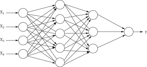
In the deep neural network, the model construction has strong structural characteristics [10]. The interface of the network model is the input layer, and the data enters the entrance of the model. When the data passes through the input layer, it enters the hidden layer. The hidden layer is not only one layer, but also the data passes through the transformation and calculation of multiple hidden layers, and the final results are transmitted to the output layer to get the final information.

This model is usually related to directed acyclic graphs. The composition of functions is illustrated in Figure 2. The full length of the chain is defined as the depth of the model. In practice, the problem is usually linearly inseparable, which requires nonlinear transformation and remapping of data distribution. The deep neural network itself undergoes multiple linear changes to build a more accurate model [11]. Get stronger learning and prediction ability.

2.1. Deep Feedforward Neural Network Structure

In the case of constructing the deep Feedforward Neural Network model [12], firstly, four basic structure layers of the model are constructed, which are input layer, two hidden layers, and output layer. Here, the input layer is mainly used for characteristic data received by the network, which is usually multidimensional data. The hidden layer extracts high-level data features from the original features. The output layer literally outputs the prediction results of the whole model, but the prediction results are mainly a simple normalized analysis of the data processed by the previous hidden layer, and the obtained output is regarded as the prediction value of the whole network. The Softmax function is used as the output of a variety of classifiers.

The formula for the sum of squared errors is as follows:

()

where o_k = f(net_k) is the actual output value of neuron k in the output layer; d_k is the expected output value of the output layer neuron k; and y_j is the output value of hidden layer neuron j.

For the E value, in order to achieve the goal of the ideal value, it is necessary to change the weight value of the network. First, adjust the connection weights between the implicit layer and the output layer.

()

In the above formula, the value obtained by the gradient method is the adjusted value of the connection weight between the implicit layer and the output layer.

()

In the above formula, η is the normal value, which is expressed as the iteration step.

Formula adjustment

()

In the above formula, the adjustment amount of the connection weight between the input layer and the implicit layer is determined by the gradient method. It can be obtained from the following formula:

()

2.2. Activation Function

According to the needs of solving practical problems, we should consider the different characteristics of various activation functions to choose flexibly. The general activation functions are Sigmoid [13], Tanh [14], and ReLU [15].

The expressions for Sigmoid and Tanh are

()

In the calculation, the hidden middle layer selects ReLU as the activation function, and the form of ReLU activation function is as follows:

()

However, when the input of ReLU activation function is negative, the gradient is still zero. To solve this problem, ReLU is improved, and its expression is

()

2.3. Loss Function

After constructing the deep Feedforward Neural Network model, it is the key to determine the loss function when backpropagating on the network. As the name suggests, the difference between the predicted value and the actual value of the output of the neural network is measured by measuring the loss function, which in turn spreads the error and improves the prediction performance after data processing. The difficulty of loss function optimization depends on the parameters, and the final model parameters are also different, so it is necessary to choose appropriate loss parameters for specific problems.

The square loss function is often used in the task of predicting that the tag y is a real value, and the formula is as follows:

()

In the multi-classification, the cross-entropy loss function is used, and the formula is as follows:

()

Crossentropy always depends on Sigmoid. When Sigmoid approaches the derivative of 1 or 0, Sigmoid becomes slack and gradient-based learning becomes particularly slow. Using crossentropy, because the derivative of the output layer is differential linear, there is no problem that the learning speed is too slow at the beginning.

2.4. Optimization Algorithm

After determining the loss function, the model has all the functional structures for data processing [16]. Next, we need to determine the optimization algorithm when the model is backpropagated. There are different operation forms such as Adam method, random gradient descent method, and batch gradient descent method. As the name indicates, the batch gradient descent method repeats all samples of the network model to update the network weight, which greatly increases the calculation amount of network data and reduces the backpropagation speed of network errors. The stochastic gradient descent method repeats only one sample of the input samples of the network model to update the weight, so as to improve the operation speed of the network and reduce the computation. However, due to the lack of repeated data, the accuracy of the network model decreases, and the final result is a local optimal solution, and the global optimal solution cannot be obtained. Therefore, the Adam method, which combines the advantages of inertia maintenance and environment perception, is adopted in the model proposed for college students’ employment prediction. The quadratic moment of the gradient shows the ability to perceive the environment and produces adaptive learning speeds for different parameters.

2.5. Dropout and Batch Normalization Method

In the process of neural network training, we often face the problem of overfitting. That is to say, when the parameters are too large and the corresponding training data is insufficient, the loss of the model in the training group is small, but the loss in the test group is large, and the generalization ability is very poor. There are many methods to solve phishing, such as data set enhancement, parameter normalization, and dropout. The training of deep learning model is not realized by iterative calculation, but in order to achieve better training effect, it is necessary to adjust the dropout ratio by continuously adjusting and correcting the weighted attenuation coefficient and enlarging or reducing the learning rate during the training of the model. The change of parameters has a great influence on the model and leads to the change of the accuracy of prediction results. As a model optimization method, the batch normalization method can minimize the negative impact of complex parameters on neural network in the process of adjusting related parameters of the model and can not only accelerate the convergence progress of the model but also improve the generalization ability of the model.

Dropout is a random strategy in depth model training and randomly discards a neuron node in neural network, because the dropout method regards it as a process of retraining neural network and can obtain a completely different network structure. Comparing the dropout method with the bagging method, because it is suitable for large-scale deep neural network training method before, it is associated with the overall model and data. In the case of large-scale network, this integration method needs calculation time. When training small batch data, the bagging method has no great advantage. Dropout, as an alternative to lightweight bagging, can implement the excellent features of bagging in a small batch of data. That is to say, the training and evaluation of neural networks are realized exponentially.

In fact, the training of data by neural network model is mainly to learn the distribution mode of data, so as to reflect certain coefficients and parameters. However, if the model training is mainly conducted from the perspective of training set and the data distribution schemes of test set and training set are obviously different, the final model is likely to be invalid; that is, the generalization ability of the model is low. Therefore, before training the model, the data should be normalized first. However, the subtle changes of each hidden layer in the neural network model affect the output of the last layer; that is, the changes of parameters of each hidden layer affect the parameters of the output layer, and the data distribution of each training set also changes. This makes the neural network model fit different data distributions during each calculation. Dropout and unified normalization methods are used after the hidden layer. For all connected deep neural networks, any neurons in each layer are in the same configuration; that is, the input and output of each neuron are the same. In this case, there must be no difference between forward propagation and backward propagation. Because the final value is the same as that of neurons at the same level, in order to avoid this phenomenon, their values are randomized at the beginning of model training, thus breaking the symmetry of this value.

2.6. Softmax Function

Neural network/deep learning is essentially a machine learning problem. In life, we apply more things and supervise learning. Taking neural network as an example, the learning result, that is, the output value Y of the output layer, can be a continuous value without range restriction or a value with discrete range restriction. Therefore, for different problems, the design of the output layer, that is, the design of activation function, should be different. Usually, in classification problems, the activation function of the output layer is generally used as the Softmax function. The Softmax function is defined as follows:

()

2.7. Algorithm Flow

In order to realize employment prediction applicable to deep neural network, Figure 3 shows the calculation flow based on deep neural network. The main process is to preprocess the data set first and then convert all types of features into numerical features with one-hot code. Secondly, the feature data of the training set is used to train the deep neural network, and the test set is used to verify the training results, and the grid search method is used to find the best parameter combination.

3. Dimension Analysis and Data Preparation of College Students’ Employment Destination

3.1. Basis for Formulating the Impact Dimension of College Students’ Employment Destination

According to the six aspects of the comprehensive quality evaluation system of college students: academic quality evaluation, character evaluation, stylistic quality evaluation, psychological quality evaluation, innovative quality evaluation, and ability quality evaluation, as well as the career development direction of college students adopted by Yuan Jiaqian, comprehensively determine the influence of this study.

3.2. Data Preparation

3.2.1. Scope of Study and Data Acquisition

Taking 853 students from 2010 to 2018 in a university as objects, according to the influence dimensions of the above six career development directions, the comprehensive data and personal technical information data of 853 students in school for 4 years were collected as data samples of this experiment.

3.2.2. Data Preprocessing

The data preprocessing stage is divided into the next step.

(1)
Data cleaning. The initial data is disorganized, with many duplicate or invalid attributes, and all the attributes of the student data table do not necessarily need to be further cleaned, as shown in Table 1
(2)
Data integration

(3)
Data conversion. In order to standardize various attribute values, this paper develops an automatic data conversion tool based on the data coding rules of the Feedforward Neural Network, which can operate various attributes more conveniently. English proficiency is measured by CET test scores. Failure to pass the CET test is indicated by 0, passing the CET4 test is indicated by 2, and passing the CET6 test is indicated by 4. The six graduation attributes of employment, further studies, going abroad, freelancing, unemployed, and not graduating are converted into 000000, 000000, 01000, and 100000, respectively, according to the algorithm code rules

Table 1. Annual data information table of a certain student (part).

Serial number	Credit grade point	English proficiency	Political civilization	Scientific and technological innovation	Stylistic art	Social voluntary service	Destination of graduation
001	1438	0	7.7954	0.9	2.41	0.3	Employment
002	1385	0.2	5.3766	0	0.3	0	Enter a higher school
003	1465	0.4	8.227	7.98	3.5	0.35	Employment
004	1773	0.2	6.9804	0	1.86	0	Employment
005	1712	0.2	5.0885	0	0.5	0	Employment
006	1634	0.2	7.0122	7.41	0.3	0.15	Employment
007	1523	0.2	4.546	4.06	0.32	0	Enter a higher school
008	1376	0.2	6.0564	0	3.92	0	Employment
009	1474	0.4	4.9983	0.2	0.35	0	Unemployed
010	1746	0.2	8.6782	4.87	2.9	0.3	Employment

The score of credits is the total score of students’ grades in 4 years, as shown in Tables 2 and 3.

Table 2. Attribute values and conversion comparison table.

Attribute value and conversion comparison table
	Attribute name	Characteristic value	Conversion value
Basic characteristics	Credit grade point
	English proficiency	Failed CET, CET4, CET6	0, 2, 4
	Political civilization
	Scientific and technological innovation
	Stylistic art
	Social volunteering
Predictive characteristics	Destination of graduation	Employment	000001
		Enter a higher school	000010
		Go abroad	000100
		Freelance	001000
		Unemployed	010000
		Not graduated	100000

Table 3. Information table fragments after data conversion.

Credit grade point	English proficiency	Political civilization	Scientific and technological innovation	Stylistic art	Social voluntary service	Destination of graduation	Category
1438	0	8	1	2	3	000001	1
1385	2	5	0	0	0	000010	2
1465	4	8	8	4	3	000001	1
1773	2	7	0	2	0	000001	1
1712	2	5	0	1	0	000001	1
1634	2	7	7	0	2	000001	1
1523	2	5	4	0	0	000010	2
1376	2	6	0	4	0	000001	1
1474	4	5	0	0	0	010000	5
1746	2	7	5	3	3	000001	1

3.3. Set the Evaluation Index of Prediction Model

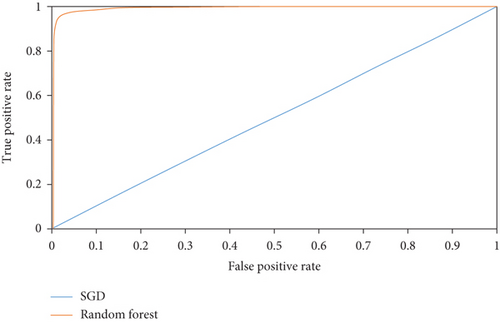
ROC curve can reflect the effect of classifiers to some extent, but it is still unclear. On the other hand, the Acc curve of the Acc evaluation model makes up for the deficiency of the ROC curve. As shown in Figure 4, the value of Acc is actually the size of the area of the ROC curve surrounded by the X-axis. This value intuitively represents the prediction effect. The smaller the value, the worse the prediction effect.

Acc values are calculated by

()

That is, the value of Acc represents the proportion of the number of correctly predicted samples to the total number of samples. The criteria for evaluating the prediction model with the Acc value are as follows:

(1)
Acc = 1, perfect
(2)
Acc = [0.8, 0.95], the effect is very good
(3)
Acc = [0.7, 0.8], the effect is average
(4)
Acc = [0.5, 0.7], the effect is low
(5)
Acc = 0.5, the prediction effect is the same as random guess

In the prediction model, the deviation between the predicted value and the actual value of a single sample is loss. In order to evaluate the degree of deviation and error between the actual value Y and the predicted value F(x), the loss function is often used. The smaller the function value, the better the robustness of the prediction model. If it is reflected in the image, the closer the loss curve is to the X-axis, the better. The loss value is calculated as follows:

()

where W represents the model parameter.

4. Experiment

4.1. Estimation of Predictive Model Algorithms

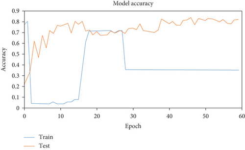
As shown in Figure 5, the Acc values of the test set and the training set are stable at about 0.74 and 0.85, respectively.

As shown in Figure 6, the loss values of the test set and the training set are stable at about 0.4 and 0.3, respectively.

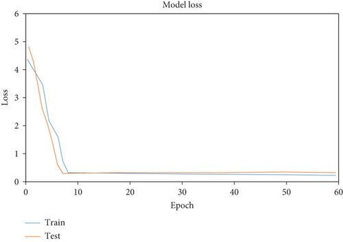
Acc value and loss value of the prediction model prove that the prediction model has better prediction effect and in-depth research and optimization experiments can be carried out in the next stage.

4.2. Model Parameter Adjustment and Prediction

4.2.1. Training Process Analysis

The deep Feedforward Neural Network is applied to classify the employment of college graduates. Figures 7 and 8 show the curves of classification accuracy and loss function with iteration times in the training and testing process of students’ employment data sets.

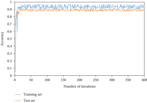
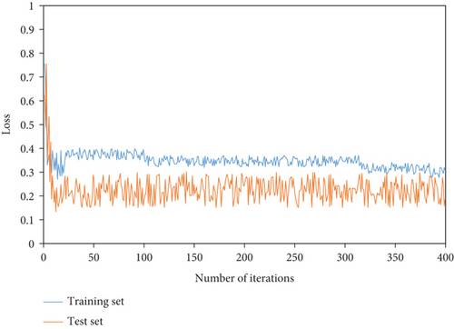
As can be seen from Figure 7, the accuracy of the training set of the employment data set increases rapidly before 20 iterations, and then, the shock of the training set decreases until it tends to be stable after 250 iterations. The test set rises rapidly before 15 iterations and then rises slowly and tends to be stable. As can be seen from Figure 8, the loss of the training set decreases rapidly in oscillation before 250 iterations and then gradually stabilizes; the test set loss decreases rapidly before 300 iterations and then decreases slowly and tends to be stable.

4.2.2. Parameter Analysis of Different Training Batch Sizes

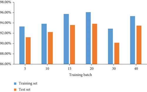
The selected training batch sizes are 5, 10, 15, 20, 30, and 40, and the training results are shown in Figure 9. The accuracy of the training set was 93.14%, 93.68%, 95.57%, 95.91%, 92.74%, and 95.13%, respectively. The accuracy of the test set was 91.14%, 92.12%, 93.44%, 93.69%, 90.09%, and 93.33%, respectively. That is, when the deep neural network selects the batch size of 20 on the data set, the accuracy of the training set reaches the highest, which is 95.91%, and the accuracy of the test set reaches the highest, which is 93.69%.

4.2.3. Model Prediction

The highest prediction accuracy of single item is “employment,” while the prediction result of “unemployed” is the worst, as shown in Table 4.

Table 4. Single forecast results of employment destination.

Career development direction	Forecast sample number	Actual sample number	Accuracy rate of single prediction
Employment	411	391	94.9%
Enter a higher school	242	262	92.4%
Go abroad	48	55	87.3%
Freelance	29	34	85.3%
Unemployed	41	35	82.8%
Not graduated	11	5	52.1%

4.3. Comparison with Traditional Prediction Algorithm

On the above-mentioned employment data set of college graduates, the deep Feedforward Neural Network model proposed in this paper, random forest, gradient lifting decision tree, and support vector machine are used for training and prediction.

The deep Feedforward Neural Network model is visually aligned with random forest, gradient lifting decision tree, and support vector machine, as shown in Figure 10.

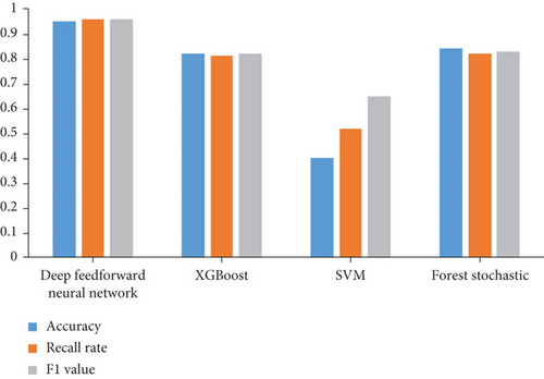
According to the comparison between the above-mentioned prediction model of college students’ employment destination based on the deep Feedforward Neural Network and random forest, gradient lifting decision tree, and support vector machine model in Figure 10, it can be seen that the deep Feedforward Neural Network model is superior to other models in terms of accuracy, recall rate, and F1 value.

5. Conclusion

Based on deep learning and Feedforward Neural Network technology, this paper establishes a prediction model of college students’ employment destination based on six evaluation dimensions and evaluates the prediction accuracy of the model. Acc value and loss value are used as indicators to test whether the prediction effect of the prediction model is good. Finally, combined with the actual data of graduates, the practical application of the prediction model is analyzed, and the effectiveness of the algorithm is verified by comparing with the traditional machine learning algorithm.

Conflicts of Interest

The author declared that there are no conflicts of interest regarding this work.

Open Research

Data Availability

The experimental data used to support the findings of this study are available from the corresponding author upon request.

References

1 Alroughani R., Alhamdan F., Shuaibi S., Ahmed S. F., Behbehani R., Lamdhade S., and Al-Hashel J., The prevalence of multiple sclerosis continues to increase in Kuwait, Multiple Sclerosis and Related Disorders. (2019) 32, 74–76, https://doi.org/10.1016/j.msard.2019.04.033, 2-s2.0-85064926190, 31055174.
10.1016/j.msard.2019.04.033
CAS PubMed Web of Science® Google Scholar
2 Sun W., Wang N., and Shen L., The relationship between employment pressure and occupational delay of gratification among college students: positive psychological capital as a mediator, Current Psychology. (2021) 40, no. 6, 2814–2819, https://doi.org/10.1007/s12144-019-00209-w, 2-s2.0-85062774229.
10.1007/s12144-019-00209-w
Web of Science® Google Scholar
3 Chang Y.-p., Developing students' ability to solve word problems through learning trajectory-based and variation task-informed instruction, Mathematics Education. (2019) 51, no. 1, 169–181, https://doi.org/10.1007/s11858-018-0983-8, 2-s2.0-85059845965.
10.1007/s11858-018-0983-8
Google Scholar
4 Abd A. M., Hameed A. H., and Nsaif B. M., Documentation of construction project using integration of BIM and GIS technique, Asian Journal of Civil Engineering. (2020) 21, no. 7, 1249–1257, https://doi.org/10.1007/s42107-020-00273-9.
10.1007/s42107-020-00273-9
Google Scholar
5 Li D., Deng L., and Cai Z., Research on image classification method based on convolutional neural network, Neural Computing and Applications. (2021) 33, no. 14, 8157–8167, https://doi.org/10.1007/s00521-020-04930-7.
10.1007/s00521-020-04930-7
Web of Science® Google Scholar
6 Liu H., Gao Q., and Ma P., Photovoltaic generation power prediction research based on high quality context ontology and gated recurrent neural network, Sustainable Energy Technologies and Assessments. (2021) 45, no. 16, article 101191, https://doi.org/10.1016/j.seta.2021.101191.
10.1016/j.seta.2021.101191
Web of Science® Google Scholar
7 Seleq S., Jo E., Poole P., Wilkinson T., Hyland F., Rudland J., Verstappen A., and Bagg W., The employment gap the relationship between medical student career choices and the future needs of the New Zealand medical workforce, The New Zealand Medical Journal. (2019) 132, no. 1506, 52–59.
PubMed Web of Science® Google Scholar
8 Alfarozi S. A. I., Pasupa K., Sugimoto M., and Woraratpanya K., Local sigmoid method: non-iterative deterministic learning algorithm for automatic model construction of neural network, IEEE Access. (2020) 8, 20342–20362, https://doi.org/10.1109/ACCESS.2020.2968983.
10.1109/ACCESS.2020.2968983
Web of Science® Google Scholar
9 Ding D., Liu Z., Zhang H., Xu J., and Wu J., Synthesis, topological structure and magnetism of a scarce homochiral octanuclear metallarectangle, Inorganica Chimica Acta. (2021) 519, no. 404, article 120281, https://doi.org/10.1016/j.ica.2021.120281.
10.1016/j.ica.2021.120281
Web of Science® Google Scholar
10 Du X., Li Z., Ma Y., and Cao Y., Efficient network construction through structural plasticity, IEEE Journal on Emerging and Selected Topics in Circuits and Systems. (2019) 9, no. 3, 453–464, https://doi.org/10.1109/JETCAS.2019.2933233, 2-s2.0-85070679891.
10.1109/JETCAS.2019.2933233
Web of Science® Google Scholar
11 Guo D. and Lin X., Li-function activated Zhang neural network for online solution of time-varying linear matrix inequality, Neural Processing Letters. (2020) 52, no. 1, https://doi.org/10.1007/s11063-020-10291-y.
10.1007/s11063-020-10291-y
Web of Science® Google Scholar
12 Aggarwal A., Vinayak V., Bag S., Bhattacharyya C., Waghmare U. V., and Maiti P. K., Predicting the DNA conductance using a deep feedforward neural network model, Journal of Chemical Information and Modeling. (2021) 61, no. 1, 106–114, https://doi.org/10.1021/acs.jcim.0c01072, 33320660.
10.1021/acs.jcim.0c01072
CAS PubMed Web of Science® Google Scholar
13 Ren N., Fan L., and Zhang Z., Sensorless PMSM control with sliding mode observer based on sigmoid function, Journal of Electrical Engineering & Technology. (2021) 16, no. 2, 933–939, https://doi.org/10.1007/s42835-021-00661-4.
10.1007/s42835-021-00661-4
Web of Science® Google Scholar
14 Piao X. and Kim P., The modified extended tanh-function method for solving Burgers-type equations, Physica A: Statistical Mechanics and its Applications. (2021) 569, no. 4, article 125771, 394–404, https://doi.org/10.1016/j.physa.2021.125771.
10.1016/j.physa.2021.125771
Web of Science® Google Scholar
15 Eckle K. and Schmidt-Hieber J., A comparison of deep networks with ReLU activation function and linear spline- type methods, Neural Networks. (2019) 110, 232–242, https://doi.org/10.1016/j.neunet.2018.11.005, 2-s2.0-85059446493, 30616095.
10.1016/j.neunet.2018.11.005
PubMed Web of Science® Google Scholar
16 Chen G., Wang L., and Kamruzzaman M. M., Spectral classification of ecological spatial polarization SAR image based on target decomposition algorithm and machine learning, Neural Computing and Applications. (2020) 32, no. 10, 5449–5460, https://doi.org/10.1007/s00521-019-04624-9.
10.1007/s00521-019-04624-9
Web of Science® Google Scholar

Citing Literature

All articles

[Retracted] Employment Data Screening and Destination Prediction of College Students Based on Deep Learning

Retraction(s) for this article

Retracted: Employment Data Screening and Destination Prediction of College Students Based on Deep Learning

Abstract

1. Introduction

2. Deep Feedforward Neural Network