Dynamical Behaviours of Stage-Structured Fractional-Order Prey-Predator Model with Crowley–Martin Functional Response
Abstract
In this paper, the dynamic behaviour of the stage-structure prey-predator fractional-order derivative system is considered and discussed. In this model, the Crowley–Martin functional response describes the interaction between mature preys with a predator. The existence, uniqueness, non-negativity, and the boundedness of solutions are proved. All possible equilibrium points of this system are investigated. The sufficient conditions of local stability of equilibrium points for the considered system are determined. Finally, numerical simulation results are carried out to confirm the theoretical results.
1. Introduction
The subject of fractional integral and derivative is as old as classical calculus. This type of calculus is more comprehensive than the differ-integral calculus due to its worldwide applications in biology as well as in different branches of science, engineering, several ecological models, and some other interdisciplinary fields [1–4]. Many researchers have performed and investigated models of fractional derivatives [5, 6]. Some types of fractional derivatives like Caputo, Caputo–Fabrizio, Riemann–Liouville, and Marchand are powerful mathematical tools for modelling biological systems which cannot be designed by integer derivatives because fractional-order derivatives are not only dependent on the initial conditions but also on the memory of the system [7, 8]. The Lotka–Volterra equations are the first equations that described the dynamics of biological systems, which are also called the predator-prey equations. A stage-structured predator-prey model is considered and elucidated by the authors in Reference [9]. Some authors [10–16] have studied two species models with stages structured in the predators. They discussed and investigated the stability of the all equilibrium points as well as the dynamic behaviour of their systems. In recent years, the global and local dynamics behaviour of a stage-structured predator-prey model is investigated, and the optimal control of harvesting is discussed in References [17–20]. The predator-prey functional response is very important to determine the relationship between the predator and prey for that there are many types of functional responses, namely, Holling types I, II, III, and IV; Michaelis–Menten ratio-dependent type; and Beddington–DeAngelis type of them have been considered and analysed in References [21–27]. The Crowley–Martin functional response is simplified to Michaelis–Menten which has involved one more term explaining mutual interferences of predators for the case where the predator feeding rate is decreased by a higher predator density even when the prey density is high [28, 29]. The subject of the optimal harvesting is very important in managing the renewable resources due to the economic aspect and to keep population at level far from the extinct, so that many researchers and authors have widely investigated and studied this subject in their works, see [30–34] and the references therein.
In this work, we have considered and developed a fractional-order with the Caputo fractional derivative model for a stage-structured prey-predator model with Crowley–Martin functional response and linear harvesting for mature prey species only. The current paper is divided as followsSection 2 contains the main definitions of fractional derivatives and theories for the local stability of the equilibrium points that are used throughout this work. In Section 3, the model is formulated with the existence of all its equilibria. The existence and boundedness of its solution are proved and shown. In Section 4, the conditions for the local stability of all equilibrium points are established. Section 5 presents and confirms the numerical simulation for the theoretical results, while the conclusions and discussions are given and elucidated in Section 6.
2. Main Concepts
Definition 1. (see [35, 36]). The fractional-order derivatives in the meaning of Caputo are defined as follows:
Some results for the fractional-order derivatives are found in References [21, 25, 37] that are needed throughout this paper.
Lemma 1. Assume that f(t) ∈ C[a, b].
- (1)
-
where a ≤ ζ ≤ sfor alls ∈ (a, b]
- (2)
If , then we have:
- (i)
If for allt ∈ (a, b), thenf(t)is a nondecreasing function for all t ∈ [a, b].
- (ii)
If for allt ∈ (a, b) then f(t)is a nonincreasing function for allt ∈ [a, b].
- (i)
Lemma 2. Assume the Cauchy problem.
In the autonomous case:
Then, the solution is h(t) = bEq[λ(t − a)q] and Eq is the Mittag-Leffler function.
Lemma 3 (see [21].)Let w(t) be a continuous function on [t0, ∞) and satisfies
, then the form of the solution of this equation is given by:
The next lemma is found in Reference [38] which gives the uniqueness of the solution of fractional-order system.
Lemma 4. Let be a system fractional-q-order derivatives with the initial condition . Then, the above system has a unique solution on [t0, ∞) × Ω if f(t, u) satisfies the locally Lipchitz condition concerning u.
To examine the stability of the fractional-order system, we need the following.
Definition 2. (see [39]). Let f(x) = xn + vn−1xn−1 + vn−2xn−2 + ……+v0 be a polynomial of degree n, then the discriminant of f(x) denoted by D(f) is defined by D(f) = (−1)n(n − 1)/2R(f, f′), where f′ is the derivative of f and g(x) = xn + kn−1xl−1 + kn−2xl−2 + ……+k0 and R(f, g) are (n + l) ⊗ (n + l) determinants.
Lemma 5 (see [39].)Consider a characteristic polynomial equation, f(λ) = λn + vn−1λn−1 + vn−2λn−2 + …….. + v0, then:
- (1)
If n = 2, then the conditions for |argλi| > qπ/2, for i = 1,2 q ∈ (0,1) are either Routh–Hurwitz conditions or and
(7) - (2)
If n = 3, then we have the following cases:
- (i)
- (ii)
If D(f) < 0, v2 ≥ 0, v1 ≥ 0, v0 > 0, then|argλi| > qπ/2 i = 1, 2, 3 for q < 2/3.
- (i)
3. The Fractional-Order Model
X1(T), X2(T) are the densities of immature and mature prey species, respectively. Y1(T)andY2(T) represent the densities of immature and mature predator species respectively. The parameter R is the birth rate of immature prey; B and H1 indicate maturity rate of immature prey and immature predator, respectively; B1 and B2 express the competition rate between a mature prey population and mature predator population, respectively; D1, D2, D3, D4 are the death rates of immature and mature prey, the death rates of immature and mature predators, respectively. A1 is the maximum value which per capita reduction rate of the mature prey can attain, while A2 is the predator conversation rate. α and β are measures of the half-saturation of prey species and the coefficient of interference among predators at a high density of mature prey, respectively. All that parameters are positive.
With x1(t) ≥ 0, x2(t) ≥ 0, x3(t) ≥ 0.
The following theorem gives the boundedness and non-negativity of the solution of the system (13).
Theorem 1. For the fractional-order system (13), we have the following:
- (1)
All solutions that start in F+ = {(x1, x2, x3) ∈ ℝ3|x1 ≥ 0, x2 ≥ 0, x3 ≥ 0} are non-negative solutions.
- (2)
If 1 + b > rd1/d2, then all solutions that start in F+ are bounded.
Proof.
- (1)
To prove the solution of the fractional-order system (13) is nonnegative, we start with x1(0) > 0fort = 0 assuming that x1(t) ≥ 0, fort ≥ 0 is not true; therefore, there exists t∗ > 0 such that
(14) -
So, from the first equation of the system (13), we obtain the following:
(15) -
According to part (1) of Lemma 1, we get and this is contradiction because .
-
Therefore, x1(t) ≥ 0, for allt ≥ 0. In the same manner, we can prove that x2(t) ≥ 0, x3(t) ≥ 0, for allt ≥ 0.
- (2)
Let F+ = {(x1, x2, x3) ∈ ℝ3|x1 ≥ 0, x2 ≥ 0, x3 ≥ 0}, and x1, x2, and x3 in ℝ3, define a function Vt = x1(t) + r/d2x2(t) + ra1/d2a2ra1/d2a2x3(t), it follows that
(16) -
Now, for each k> 0, we have
(17) -
If we choose k < min{1 + b − rd1/d2, h, d3}, then we get DqV(t) + kV(t) ≤ ε for some ε > 0.
Then, from Lemma 3, we obtain that V(t) ≤ (V(0) − (ε/k))Eq[−k(t − 0)q] + v/K. Therefore, we have 0 ≤ V(t) ≤ ε/k as t⟶∞ and all solutions of system (13) are bounded.
The next theorem gives the existence and uniqueness of the solution system (13).
Theorem 2. The existence and uniqueness solution of system (4) are given for each non-negative initial condition:
Proof. Let the region be defined by F × (0, T], T < ∞.
Where .
We assume that = and B(X) = (B1(X), B2(X), B3(X)) be a mapping, such that
For , one can get the following:
Since , we have.
Where L = max{1 + b + d1, (r + d2 + h + a1 + a2)(M(1 + M)), (d3 + (a1 + a2)M(1 + M))}. Therefore, B(X) satisfies the Lipchitz condition, so that the system (4) has a unique solution.
4. Local Stability Analysis
In this section, we investigate the existence of the equilibrium points of the system (4). We also give the conditions for the local stability of its equilibria.
Theorem 3 (see [41], [42].)Consider the following fractional-order differential system:
, q ∈ (0,1), and . The point that satisfies is called the equilibrium point of the system (20). It is called locally asymptotically stable if |arg(λi)| > qπ/2 for i = 1,2, …..n, where λi are the eigenvalues of the Jacobian matrix which are evaluated at . Otherwise, it is called an unstable point.
To find all possible equilibrium points of the system (4), we have to solve the following equations:
Therefore, the system (4) has three possible equilibrium points, namely:
- (1)
The trivial equilibrium point e0 = (0,0,0) always exists.
- (2)
The free predator point exists if
(22) - (3)
The interior exists only if
(23) -
where = ( is the positive root of the following equation:
(24) -
Here, a = a1d3 − a1a2 + a2(d1r/1 + b–d2 − h)/a1d3 and b1 = a2(d1r/1 + b − d2 − h)/a1d3.
Since b1 > 0ifa < 0 then, equation (24) may have two positive real roots.
The Jacobian matrix of fractional-order system (4) associated with arbitrary fixed point (x1, x2, x3) is given by
So, the general characteristic equation of (25) is as follows:
To analyse the local stability of the fixed points e0, e1, e2, we give the following theorem.
Theorem 4. For the system (4), we have the following:
- (1)
If d2 + h + bd2 + bh > rd1, then the point e0 is a locally stable point.
- (2)
The free predator point e1 is always an unstable point.
- (3)
The interior equilibrium pointe2 is locally asymptotically stable if one of the following conditions hold.
- (i)
If D(f) > 0, p2 > 0, p0 > 0 and p1p2 > p0for q ∈ (0,1).
- (ii)
If D(f) < 0, p2 ≥ 0, p1 ≥ 0, p0 > 0 for q < 2/3, where p2, p1, and p0 are defined in equation(29).
- (i)
Proof.
- (1)
For the point e0, the Jacobian matrix J(e0) is given as follows:
(29) -
So, the characteristic equation is P(λ) = (−d3 − λ)(λ2 + u1λ + u0).
-
Where u1 = (1 + b + d2 + h) and u0 = (d2 + h + bd2 + bh − rd1). The roots of the above characteristic equation are λ1 = (−d3). It is clear that |argλ1| = π > qπ/2.
-
Since u1 > 0 and if d2 + h + bd2 + bh > rd1 that means u0 > 0, then the Routh–Hurwitz conditions are satisfied.
-
According to part 1 of Lemma 5, e0 is stable.
- (2)
It is clear that the Jacobian matrix J(e1) is as follows:
(30) -
And the corresponding characteristic equation is as follows:
(31) -
Therefore, one of the eigenvalues is equal to zero. Thus, the free predator pointe1 is unstable.
- (3)
The Jacobian matrix at the interior equilibrium pointe2 is given as follows:
(32) -
So, the characteristic polynomial of J(e2) can be obtained:
(33) -
where
(34) -
Then, the discriminant D(f) of the cubic polynomial f(λ) is the following:
(35)
According to Lemma 5 (2), if D(f) > 0, p2 > 0, p0 > 0 and p1p2 > p0for q ∈ (0,1), or D(f) < 0, p2 ≥ 0, p1 ≥ 0, p0 > 0 for q < 2/3.
Then, the interior fixed point e2 is locally asymptotically stable.
5. Numerical Simulations
In this section, we give numerical simulations to confirm the theoretical results that are employed in Section 4. For the equilibrium point e0, the parameter values in Table 1 are considered to carry out that e0 is locally asymptotically stable. Figure 1 shows that e0 is locally stable according to conditions in Theorem 4.
| Parameter | Parameter value |
|---|---|
| d1 | 0.1 |
| b | 0.2825 |
| h | 0.1 |
| d3 | 0.5133 |
| r | 6.2416 |
| a2 | 0.5851 |
| d2 | 0.9872 |
| a1 | 0.6621 |
| q | 1,0.98, 0.88, 0.78 |
| x1(0) | 0.4175 |
| x2(0) | 1.9799 |
| x3(0) | 0.837 |
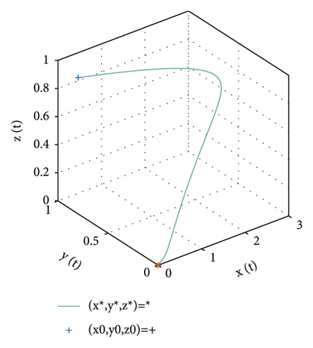
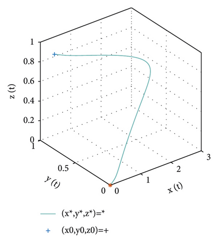
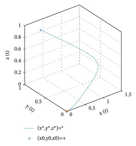

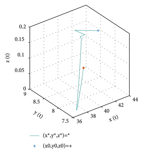
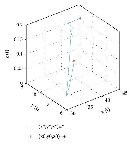
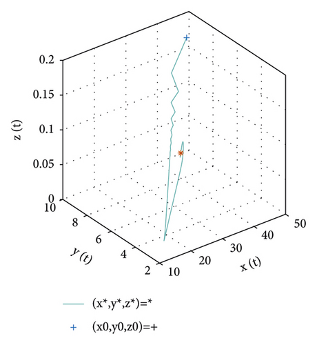
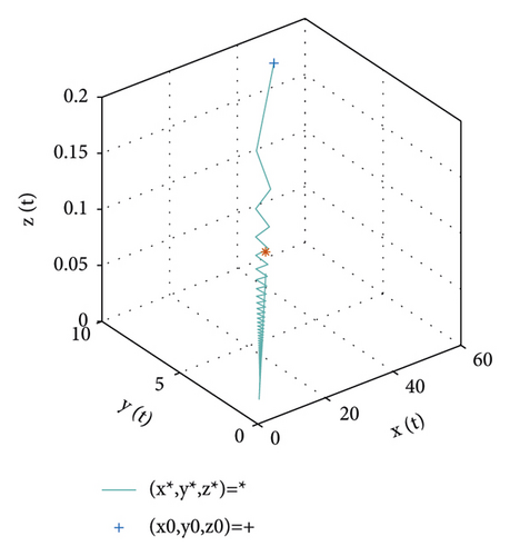
For the equilibrium point e2, the values of parameter are chosen and set in Table 2. According to the conditions in Theorem 4, the point e2 is locally stable. Figure 2 illustrates the stability of the positive equilibrium point e2.
| Parameter | Parameter value |
|---|---|
| d1 | 0.3299 |
| b | 0.2825 |
| h | 0.6168 |
| d3 | 0.5133 |
| r | 6.2416 |
| a2 | 0.5851 |
| d2 | 0.9872 |
| a1 | 0.6621 |
| q | 1, 0.98, 0.88, 0.78 |
| x1(0) | 41.6 |
| x2(0) | 8 |
| x3(0) | 0.2 |
6. Conclusions
The fractional-order differential system has been successfully applied in mathematical biology. In this paper, we have discussed the dynamical behaviour of a stage-structure prey-predator with Crowley–Martian functional response and a linear harvesting rate in a fractional-order state. The existences, uniqueness, non-negativity, and the boundedness solutions of the fractional-order system are presented and proved. It is found that the considered system has at least three equilibrium points. One of them are unstable points. For the other points, conditions are set to guarantee their local stability.
Conflicts of Interest
The authors declare that they have no conflicts of interest.
Open Research
Data Availability
The data used to support the findings of this study are available from the corresponding author upon request.


