Since the 1990s, emerging market financial crises have occurred frequently, causing huge damage to the real economy, and if we cannot find effective means of early warning and prevention of financial crises, the entire international economy and society will bear the high costs of crisis management. Difference nonparametric test and Spearman nonparametric correlation analysis were carried out with cash flow financial data, and 14 financial indicators with strong discriminant ability were selected from 28 financial indicators as the input variables of the model. Due to the limitations of traditional statistical methods, a BP neural network financial distress early warning model is established. Finally, a particle swarm optimization BP neural network financial early warning model is established for the shortcomings of the BP network. These 14 indicators can have strong information timeliness. The prediction accuracy rates of the two early warning models for the test samples are 80% and 85%, respectively. The empirical results show that the two models have good prediction effects. The prediction effect of the swarm optimization BP neural network model is better than that of the BP neural network model. Therefore, the particle swarm optimization BP neural network model proposed in this paper is suitable for solving the problem of discrimination and prediction of the financial distress of enterprises. The company’s financial distress early warning has good application prospects and application value. Therefore, it has very important research significance for the early warning of the corporate financial crisis.

1. Introduction

Behind the prosperity of any business, there may be a profound crisis. What is more terrible than the crisis is the unawareness of the existence of the crisis. Therefore, enterprise continuing operation crisis prediction [1] is the process of analyzing the enterprise crisis precursor, finding the root cause of the precursor, controlling the further development of the dangerous situation, or nipping the dangerous event in the bud. The purpose of crisis prediction is to reduce the occurrence of crisis or reduce the destruction degree of crisis and realize the continuous operation of enterprises. After him, a large number of researchers followed his ideas and began to conduct in-depth research on the prediction of corporate financial distress [2].

The relevant research on the prediction of enterprise financial difficulties in China is later than that in the United States because China’s financial enterprises started late. The development of the securities market has become an indispensable part of the development of my country’s market economy [3].

With the continuous development of the economy, many problems of listed companies themselves are gradually emerging:

(1)
Due to the imperfection of many laws and regulations in the market and the imperfect supervision, some companies that do not meet the listing conditions use means such as falsely reporting financial statements to package themselves to achieve the purpose of listing. It not only caused confusion in the trading market but also caused economic losses to investors [4]
(2)
Many listed companies have unbalanced internal economic structures due to poor management. So after the listing is an annual loss, there is a serious blow to investor confidence, not conducive to market stability [5]

By the end of 2020, there were 83 securities investment consulting companies, which have remained stable in recent years. In 2020, securities investment consulting institutions have registered 11,848 employees, an increase of 3,119 over the previous year, a significant increase of 35.73%. However, listed companies still have the above problems. Therefore, it is urgent to conduct in-depth research on the phenomenon of listed companies with low quality and frequent financial distress [6].

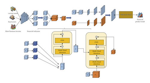
In view of this, the author believes that establishing an effective forecasting model to predict and analyze the financial status of my country’s listed companies and give early warnings can not only provide the protection of economic interests for the majority of investors but also reduce losses [7]. It can also provide more accurate early warning information for the regulatory agency China Securities Regulatory Commission, which can well avoid the probability of major economic crises and maintain good economic market order. This is also the original intention of this paper [8]. The model designed in this paper is shown in Figure 1, first screening financial indicators, and then constructing model variables to predict the financial risk of enterprises using the BP neural network.

Details are in the caption following the image — Open in figure viewer PowerPoint

2. State of the Art

Based on previous research results, Wang [9] defined financial distress as follows: from a financial point of view, financial distress includes negative net assets and the inability to repay creditor debts.

Zhu and Li believed that the financial distress of an enterprise can be defined from four aspects: first, enterprise failure, second, statutory bankruptcy, third, technical bankruptcy, and fourth, accounting bankruptcy. Zhu and Li definition essentially includes all kinds of situations from the beginning of financial distress to finally filing bankruptcy in accordance with the law, and this definition is more comprehensive and general [10].

Khouri et al. defined the operation failure of listed companies according to different research purposes as (1) enterprises unable to repay interest and principal, (2) enterprises with ROE lower than the bank interest rate, (3) ST enterprises, and (4) PT enterprises [11]. Li et al. for financial risk warning put forward the optimized BP nervous system as a financial warning model and ensure its high prediction accuracy; through the analysis of the financial risk of listed companies in 2017–2020, we found that the accuracy of the BPNN has reached more than 80% and proved the effectiveness of the BPNN optimization [12].

The financial difficulties of the P2P platform are divided into four categories, ranging from low to high, which are major bad debts, difficulties in withdrawing cash, loss of executives, and judicial bankruptcy. The second is the difficulty of the withdrawal, that is, the situation in which investors are affected by the decline in the credibility of the platform, rumored bankruptcy, and other news and collectively request a cash withdrawal.

In this article, the financially distressed company is defined as a company subject to ST (Special Treatment). Therefore, it is inappropriate to use bankruptcy to define the financial distress of Chinese listed companies at the current stage. Secondly, special handling is an objectively occurring event with high measurability [13]. The significance of special treatment is divided into other special treatments and special treatments that warn of the risk of termination of a listing. (1) Warning of the special treatment of the risk of termination of listing referred to as delisting, which includes the following: the daily upper limit of the first stock quote is 5%. The second is to add the word ∗ST before the abbreviation of the company’s stock to distinguish it from other stocks. (2) Other special treatments include the following: the daily upper limit of the first stock quote is 5%. The second is to add the word ∗ST before the abbreviation of the company’s stock to distinguish it from other stocks. There are two types of special treatments: other special treatments and special treatments for delisting risk tips. From the perspective of companies that have escaped special handling, it was only through large-scale asset reorganization that the status of ST was removed. Therefore, taking ST as a financially distressed company at the current stage is in line with the actual situation in my country [14].

3. Methodology

3.1. BP Artificial Neural Network

The artificial neural network is an information processing system formed by theoretical abstraction and simplification by simulating the structure and function of the human brain neural network in physiology and its basic characteristics [15].

Similar to the physiological neural network, the artificial neural network is also composed of a large number of artificial neurons through the rich and perfect connections of the machine [16].

In the artificial neuron structure model above, X1, X2, …, Xn are input signals, weights W1, W2 …, WN represent the connection strength of each input, θ is the internal neuron threshold, neuron output is y, and f() is an information processing function, generally called a transfer function. The relationship between the output, input, and transfer function of a neuron is shown in

()

We can get a basic understanding of BP neurons through an intuitive model. As shown in the model, R input values are, respectively, equipped with R weights W to connect to the next layer of the model [17]. The operation of the entire model can be expressed as

()

f as the transfer function is used to represent the relationship between input and output, P is the input vector, W is the weight vector, and b is the threshold vector. Figure 2 shows the BP network neuron model [18].

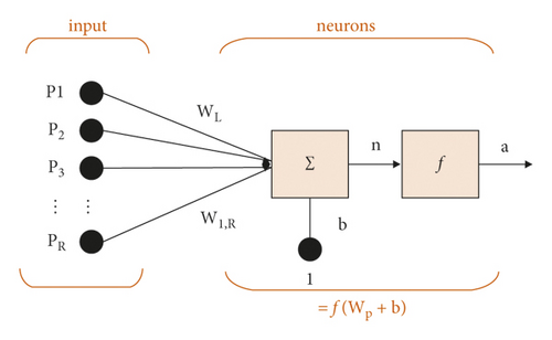
BP neural network usually has one or more hidden layers, the running connection of neurons in the hidden layer must be a sigmoid function, and the neurons with no restriction on the function type are in the output layer [19].

As shown in Table 1, it is the BP neural network model prediction and test judgment result table. The table makes a more detailed comparison between the actual number of samples and its own judgment number. It can be said that the sample collection work involved in this topic has a good guiding role [20].

1. BP neural network model prediction and test result table.

Group	Modeling samples		Test sample
Group	Actual number	Correctly determine the number of	Actual number	Correctly determine the number of
ST	60	51	30	25
Not ST	60	58	30	29
Correct decision rate (%)	90.8		90

3.1.1. Overall Structure of BP Neural Network

The input, output, weights, threshold matrix, and a hidden layer of this layer and its weights, threshold matrix, hidden layer transfer function, and output layer transfer function constitute a complete BP neural network [21].

In order to more accurately grasp the functional modules of various aspects of the BP network, the model of this subject has made statistics on the probability distribution of 70 listed companies (as shown in Figure 3).

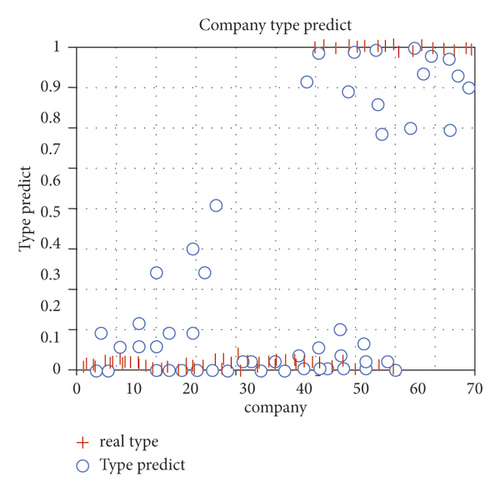
The horizontal axis of this graph represents the 71 sample companies, and the vertical axis represents the probability of financial risk. The red “+” sign represents the observed value, and the corresponding horizontal axis represents the company number. The occurrence of financial risk is “1,” and the occurrence of no financial risk is “0.” The blue “o” represents the predicted value obtained in the neural network model, and the corresponding vertical axis represents the probability of occurrence of financial risk.

From this Matlab simulation graph, it can be seen that the probability distribution of financial distress of listed real estate companies under the neural network model is concentrated on the lower side of the chart; we should make better use of the BP neural network model to serve our real life.

The test results of Matlab can accurately display the financial indicators BP neural network model discriminant test; we can clearly see the fluctuation of the observed value and the predicament value through the table. When the dilemma value fluctuates in the range of 1-1.1, the accuracy of the model prediction can reach 91.7%, while when the dilemma value fluctuates in the range of 0.9-1, the accuracy of the model prediction is only 77.3. When the fluctuation range is not considered, the total prediction accuracy of the model is 87.2%. The specific data are shown in Table 2.

2. Observations and tests of step 1.

	Observations		Inspection situation
			Dilemma value		Correct rate (%)
			0-0.1	0.9-1	Correct rate (%)
Step 1	Dilemma value	0-0.1	44	4	91.7
	Dilemma value	0.9-1	5	17	77.3
	Total correct rate				87.2

3.2. Using AdaBoost Algorithm to Optimize BP Neural Network

The BP neural network is the most widely used algorithm in the artificial upgrade network, but there are four major deficiencies in the previous section. The effect obtained is not very obvious; there is no way to get an accurate result. According to these characteristics, the AdaBoost algorithm can be used to optimize the neural network. Adaboost is an iterative algorithm, whose core idea is to train different classifiers (weak classifiers) for the same training set and then assemble these weak classifiers to form a stronger final classifier (strong classifier).

One aspect of the AdaBoost algorithm applied to upgrading the network is to optimize the structure of the artificial neural network, and the other aspect is to use the AdaBoost algorithm to learn the weights of the neural network, that is, to replace some traditional learning algorithms with the AdaBoost algorithm.

Due to its strong adaptability to the accuracy of weak classifiers, the AdaBoost algorithm is used in many machine learning processes. We combine the BP_AdaBoost theory with the upgraded network to improve the reliability of the evaluation results of the BP network.

As an iterative algorithm, AdaBoost is implemented by using different kinds of classifiers to train the same training set. These resulting weak classifiers are then aggregated, resulting in a more powerful classifier. The algorithm itself is achieved by changing the distribution of the data. The core of the AdaBoost algorithm is to eliminate unnecessary data and focus on the operation of key values.

The implementation of the AdaBoost algorithm is deduced as follows:

Define a sample space as X, and define the set of identities of sample categories as Y. Assuming this is a binary classification problem, we restrict Y to be values between positive and negative 1, and let S = {(Xi, Yi)|i = 1,2, …, m} as the sample training set, where Xi belongs to set X and Yi belongs to set Y.

(1)
In a given sample training set, the sample space and the category identification set correspond to positive and negative samples, respectively; the maximum number of training cycles is referred to as T
(2)
The initialization probability distribution of training samples is defined as 1/n
(3)
Analyze an iterative process:
- (1)
  Under the same probability distribution, perform the first training of the weak classifier
- (2)
  Analyze the error probability of the weak classifier
- (3)
  Analyze and select the threshold to reduce the error to the lowest value
- (4)
  Update the weight of the sample

After repeating the above process T times, we can obtain T weak classifiers, which are superimposed according to the updated weights to obtain the final strong classifier.

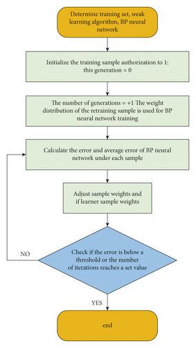
According to the above process, after T times of repetition, each operation is based on the currently obtained weight distribution, we can define a distribution P for the sample space, and then, we can obtain a weak classifier for this distribution. The rule it follows is to reduce the probability of classifier data with a good classification effect and increase the probability of classifier data with a poor classification effect. The final classifier can be obtained by the weighted average of the weak classifiers. Figure 4 shows the flowchart of its algorithm.

3.3. Regularization Method

In general, the training performance function of the neural network adopts the mean square error function E. Denote the neural network model training set D = (x, t.), where i = 1, 2, …, n, n is the total number of training samples, w is the network parameter, and m is the number of parameters. Given the network frame H and the initial values of network parameters W, the network error function is E. Take the error sum of squares:

()

Among them, y(o) is the actual output of the network, and k is the output of the neural network. Since the neural network to be designed in this paper has only one output, only the case of k = 1 is discussed; then, E can be expressed as

()

In order to overcome the overfitting problem in the network learning process, the regularization method is commonly used to add a weight decay term Ew after the error function.

()

where w is the network parameter and m is the number of parameters. So the total error function can be defined as

()

The Bayesian method comes from people’s reasoning methods for things. For deterministic things, people generally use deductive methods, and for uncertain things, they generally use inductive and inferential reasoning methods. Bayesian methods use probabilistic languages to describe things. The probability distribution used to describe the unknown case of a variable 0 before any data is obtained is called the prior distribution. The Bayesian formula can be expressed as

()

4. Result Analysis and Discussion

The model in this paper uses the optimized BP neural network model, the development of early warning models is gradually improved with the development of statistical technology, and there have been methods such as univariate discriminant models, multiple logistic regression models, artificial neural network models, and support vector machine models. The model in this paper adopts an optimized BP neural network model, which does not require independent variables to obey conditions such as multivariate normal distribution, so it is widely used at present and uses the financial index data of my country’s listed companies in year t − 1 to model and predict their financial risk status in year t. The model has a forecast lead time of 1 year.

4.1. Model Variable Structure

Financial indicators include 52 indicators in the following 6 aspects: operating capacity indicators, solvency indicators, cash flow indicators, growth capacity indicators, profitability indicators, and earnings management indicators. The detailed classification is shown in Table 3.

3. List of financial indicators to be selected.

Operational capability index	Current assets turnover ratio, fixed assets turnover ratio, net assets turnover ratio, total assets turnover ratio
Solvency indicator	Net assets to fixed assets ratio, net debt to net assets ratio, current ratio, quick ratio, conservative quick ratio, gearing ratio, equity multiplier, tangible net worth debt ratio
Cash flow indicator	Sales cash ratio, main income cash content, cash recovery rate of all assets, cash-to-liability ratio, total cash-to-debt ratio
Growth capability indicator	Year-on-year growth rate of main business income, year-on-year growth rate of main business profit, year-on-year growth rate of operating profit, year-on-year growth rate of profit before interest and tax, year-on-year growth rate of profit before tax, year-on-year growth rate of net profit, net cash flow from operating activities, year-on-year growth rate of total assets, year-on-year growth rate of return on equity, year-on-year growth rate of the net increase in cash and cash equivalents, year-on-year growth rate of total assets, year-on-year growth rate of net assets
Earnings management indicators	Net asset interest rate, return on assets, return on total assets of the core business, net sales profit margin, gross profit margin on sales, main business profit rate, main business cost rate, and period expense rate. Management expense ratio, financial expense ratio, main business profit ratio, operating profit ratio
Profitability indicator	Accounts receivable rate, accounts receivable rate change, net accounts receivable rate, net accounts receivable rate change, other accounts receivable net rate, other accounts receivable net rate change, other receivables ratio, other payable ratios, other accounts payable net ratio change limit

In this paper, the future financial risk status of listed companies that have not exposed financial risks is divided into three types: normal, loss, and ST.

We divide the selected data samples into two parts: the training set and the test set. Because the significance level of the selected 52 indicators is positioned at 0.05, it can be directly put into the actual calculation.

However, if we want to solve practical problems through the BP neural network model, we must choose the number of neurons. We use the following three formulas to choose the optimal number of hidden units for calculation.

In the following formula, K is the number of samples, n1 is the number of hidden units, and n is the number of input units; if i > n1, then inic = 0.

()

where m and n are defined as the number of output and input neurons, respectively. The value range of a is a constant between 1 and 10.

()

The number of input neurons is n.

In the selection of indicators in the next chapter, we selected 18 financial indicators as the input layer. After judgment, the value of the number of input units n is 18, and the value of the number of output neurons m is 3. According to the above design formula, then considering the actual model, we tentatively set the value n of the neurons in the hidden layer as 20, 25, 30, 35, 40, 45, and 50 into the data code for experiments, as shown Figure 5:

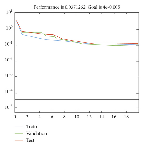
This chapter mainly lists the research plans for the lower part of the article and proposes to organically combine BP neural network with modern financial distress research, establish a corresponding data operation model, and put the data into the BP neural network model for analysis. The neural network early warning model is to apply the classification method of the neural network to financial early warning. It is analyzed from another perspective; the idea is to simulate the operation of nerves in the human brain. The method not only has good recognition ability but also has a strong self-learning ability, which can be recalculated at any time to update the data and automatically adjust the parameters, making the model more reliable. Compare the operation results with the actual results to verify the accuracy of the model. And in this chapter, which is the core department of the BP neural network, the hidden layer is organized in detail.

4.2. Model Empirical Analysis

Through selection, set A, which is the post-ST company for the modeling sample set, and set B, which is the post-ST company for the test sample, are obtained. The different sets of the two post-ST companies are due to the fact that some listed companies were ST, suspended, and resumed listing in 2009 and 2010. There are 115 listed companies in set A and 140 listed companies in set B.

From the primary selection range of sample companies, companies with negative net assets and post-ST companies are excluded, and a total of 1,207 companies in the modeling sample set and 1,176 companies in the prediction and test sample set are obtained.

The number of new ST companies and first loss-making companies in my country’s A-share market in 2007 and 2008 is shown in Table 4.

4. 2008-2009 statistical table of Class 1 and Class 2 companies.

	Class 1	Class 2	Total
2008	124	37	161
2009	158	64	222
2010	84	61	145

The number of more than 1,000 companies is too small compared to normal companies, so the modeled sample set is established in the following way: companies with a financial position of 2 in 2009 and a financial position of 2 in 2008 are combined into the ST subsample set, and the 2009 financial companies with status 1 and 2008 financial status 1 are combined into the first loss subsample set, and their financial indicators are all based on the data of the year before the year of financial status investigation; the remaining companies in the modeling sample set are determined as the normal sample set. Since the financial situation in 2008 and 2009 is normal, take the financial situation in 2009 and the financial indicator data in 2008, and make the financial situation in 2008 community, so that the empirical data is as up-to-date as possible.

For each listed company in the sample company set, the annual company financial index data constitutes an 18-dimensional vector (A1, A2, …, A18), and each element of the vector is the corresponding value of the selected financial index in the current year. The company’s financial position is represented by a three-dimensional vector: (1, 0, 0) for normal, (0, 1, 0) for the first loss, and (0, 0, 1) for ST. Since the three-dimensional vector of 0-1 has a total of eight cases, in addition to the above three cases, there are (0, 0, 0), (0, 1, 1), (1, 0, 1), (1, 1), 0), (1, 1, 1) five situations, these five situations are combined into a virtual financial situation in this paper; that is, they do not correspond to any financial risk situation.

Financial indicator data is downloaded from the BVD database.

After finishing, the modeling sample data set consists of a financial indicator matrix and a financial risk status matrix. The financial indicator matrix is a 1199 × 18 matrix (matrix A), the rows correspond to each listed company, and the columns correspond to 18 financial indicators; the financial risk status matrix is a 1199 × 3 matrix (matrix B), and each row vector corresponds to the financial risk of each listed company situation.

This paper selects only one of the two correspondences for each company when constructing the modeling sample. The selection rules are as follows: (1) if the company was ST in 2009, take 2008—>2009; (2) if the company lost money for the first time in 2008, take 2007—>2008; (3) if the company lost money for the first time in 2009, take 2008—> 2009; (4) if the company made a loss for the first time in 2008, take 2007—>2008; (5) if other companies are normal, choose 2008—>2009. The above five steps are carried out at a time. The initial selection range of companies is all 1199 companies in the overall modeling sample set. This rule ensures that each company only takes one correspondence, maximizes the sample size of ST companies and first-time loss-making companies, and uses newer data as much as possible.

The results of the prediction ability of the seven BP neural network models constructed in this paper on the financial risk status of listed companies in 2010 are shown in Tables 5 and 6.

5. BP network predicts the financial risk status of listed companies in 2010 (by the number of companies).

Number of hidden layer nodes	Type 0 companies predict the number of correct companies	0 types of companies predict the number of wrong homes	Type 1 company predicts the number of correct companies	1 type of companies predicts the number of wrong households	2 types of companies predict the correct number of companies	2 types of companies predict the number of wrong households	The number of correct predictions for all types of companies	Number of wrong predictions for all types of companies
20	913	132	5	60	43	14	961	206
25	903	142	6	59	47	10	956	211
30	915	130	7	58	44	13	966	201
35	911	134	5	60	45	12	961	206
40	909	136	4	61	47	10	960	207
45	907	138	8	57	47	10	962	205
50	903	142	7	58	46	11	956	211

6. BP Network predicts the financial risk status of listed companies in 2010 (in percentage terms).

Number of hidden layer nodes	Type 0 company forecast accuracy rate (%)	Type 0 company forecast error rate (%)	Type 1 company forecast accuracy rate (%)	Type 1 company forecast error rate (%)	Type 2 company forecast accuracy rate (%)	Type 2 company forecast error rate (%)	The prediction accuracy rate of all types of companies (%)	Prediction error rate for all types of companies (%)
20	87.37	12.63	7.69	92.31	75.44	24.56	82.35	17.65
25	86.41	13.59	9.23	90.77	82.46	17.54	81.92	18.08
30	87.56	12.44	10.77	89.23	77.19	22.81	82.78	17.22
35	87.18	12.82	7.69	92.31	78.95	21.05	82.35	17.65
40	86.99	13.01	6.15	93.85	82.46	17.54	82.26	17.74
45	86.79	13.21	12.31	87.69	82.46	17.54	82.43	17.57
50	86.41	13.59	10.77	89.23	80.70	19.03	81.92	18.08

∗ST is a company loss of three years of stocks; if the specified period can not turn around the loss, there is a risk of delisting; despite less than three years, the financial situation can also be ∗ST; in short, there is a risk of delisting of stocks. This article divides ST (including ∗ST) into two categories: A and B. The reason for Class A being ST is that the shareholders’ equity in the most recent fiscal year is lower than the registered capital. The neurological results of the last two fiscal years show that the net profit is negative, and retrospective adjustment has led to any one or more of the three consecutive losses in the last two years; the reason for Class B being ST is that the certified public accountant issued an unexpressed opinion. Audit reports with negative opinions or failure to disclose periodic reports within the statutory period.

5. Conclusion

The financial early warning model is used to study the company’s financial situation; its establishment and analysis is a process of continuous change and development and the use of the early warning model to understand the current operating conditions of enterprises and possible problems, and according to the actual changes in the model, to find the direction of development and change the investment strategy, so that the efficiency of the enterprise continues to rise. Through empirical analysis of the financial data of listed companies in my country in 2007 and 2008, this paper constructs a BP neural network model for judging the future financial crisis risk status of listed companies. The model was tested. The empirical results show that BP neural network has a strong predictive ability in predicting the financial risk status of listed companies. For normal companies and A-class ST companies, the prediction accuracy rate exceeds 80%, which is worthy of attention.

According to the empirical results of this paper, the BP neural network also has the following problems when predicting the listed companies in the whole market:

(1)
There is no predictive ability for B-type ST companies, and they are all misjudged as normal companies
(2)
The ability to predict first-time loss-making companies is low
(3)
In the case of misjudgment, they tend to misjudge first-time loss-making companies and ST companies as normal companies and tend to misjudge normal companies as ST companies
(4)
There is a situation in which the financial status of the listed company is judged to be false

The low predictive ability of the BP neural network model constructed in this paper for first-time loss-making companies is a major defect of the model. In addition, the misjudgment of false financial status does not give any substantial prediction results about the future financial status of listed companies, which is also a defect of this model.

Conflicts of Interest

The author declares that there are no conflicts of interest.

Open Research

Data Availability

The labeled dataset used to support the findings of this study is available from the corresponding author upon request.

References

1 Sun J., Fujita H., Zheng Y., and Wenguo Ai, Multi-class financial distress prediction bas ed on support vector machines integrated with the decomposition and fusion methods, Information Sciences. (2021) 559, no. 10, 225–230.
10.1016/j.ins.2021.01.059
Web of Science® Google Scholar
2 Bruno F. and Guasti L. F., A proposed corporate distress and recovery prediction score based on financial and economic components, Expert Systems with Applications. (2022) 197, no. 5, 61–70.
Web of Science® Google Scholar
3 Zhu N., Bu Y., Jin M., and Mbroh N., Green financial behavior and green development strategy of Chinese power companies in the context of carbon tax, Journal of Cleaner Production. (2020) 245, no. 4, 118908, https://doi.org/10.1016/j.jclepro.2019.118908.
10.1016/j.jclepro.2019.118908
Web of Science® Google Scholar
4 Huang W.-B., Liu J., Bai H., and Zhang P., Value assessment of companies by using an enterprise value assessment system based on their public transfer specification, Information Processing & Management. (2020) 57, no. 5, https://doi.org/10.1016/j.ipm.2020.102254.
10.1016/j.ipm.2020.102254
Web of Science® Google Scholar
5 Villar R., Olmo M., Atienza P., Garzon A. J., Wright I. J., Poorter H., and Hierro L. A., Applying the economic concept of profitability to leaves, Scientific Reports. (2021) 11, no. 1, https://doi.org/10.1038/s41598-020-79709-w.
10.1038/s41598-020-79709-w
Web of Science® Google Scholar
6 Occhino P. and Maté M., Geographical proximity on the valuations of unlisted agrarian companies: Does distance from company to company and to strategic points matter?, Agricultural Economics. (2017) 15, 6–15.
Google Scholar
7 Li D.-P., Cheng Si-J., Cheng P.-F., Wang J. Q., and Zhang H. Y., A novel financial risk assessment model for companies based on heterogeneous information and aggregated historical data, PLoS One. (2018) 13, no. 12, e0208166, https://doi.org/10.1371/journal.pone.0208166, 2-s2.0-85059220178.
10.1371/journal.pone.0208166
CAS PubMed Web of Science® Google Scholar
8 Amar J. and Samira D., Rigot Sandra Enhancing financial Transparency to Mitigate Climate change: toward a Climate risks and Opportunities reporting index, Environmental Modeling & Assessment. (2022) 27, no. 3, 46–53.
10.1007/s10666-021-09800-7
Web of Science® Google Scholar
9 Wang B., A financial risk identification model based on artificial intelligence, Wireless Networks. (2022) 28, no. 9, 112–121, https://doi.org/10.1007/s11276-021-02856-z.
10.1007/s11276-021-02856-z
CAS Google Scholar
10 Zhu L. and Li M., Metawa N financial risk evaluation Z-score model for Intelligent IoT-based enterprises, Information Processing & Management. (2021) 58, no. 6, 98–105.
10.1016/j.ipm.2021.102692
Web of Science® Google Scholar
11 Khouri S., Elexa L., Istok M., and Rosova A., A study from Slovakia on the transfer of Slovak companies to tax Havens and their Impact on the sustainability of the status of a business entity, Sustainability. (2019) 11, no. 10, https://doi.org/10.3390/su11102803, 2-s2.0-85066999838.
10.3390/su11102803
Web of Science® Google Scholar
12 Li X., Wang J., and Yang C., Risk prediction in financial management of listed companies based on optimized BP neural network under digital economy[J], Neural Computing & Applications. (2022) 9, no. 3, 20–24.
Google Scholar
13 Ery Setiawan P., I Made Pande Dwiana Putra Keputusan Pemilihan Strategi Manajemen Laba Pada Perusahaan Yang Mengalami Financial Distress di Indonesia, Jurnal Ilmiah Akuntansi Dan Bisnis. (2019) 17, no. 5, 49–61.
Google Scholar
14 Miklosik A. and Peter S., Milos Hitka Environmental sustainability disclosures in annual reports of ASX Industrials List companies, Environment, Development and Sustainability. (2021) 23, no. 11, 26–31.
10.1007/s10668-021-01338-8
Web of Science® Google Scholar
15 Sehgal S., Mishra R. K., and Jaisawal A., A search for macroeconomic determinants of corporate financial distress, Indian Economic Review. (2021) 56, no. 6, 109–117.
10.1007/s41775-021-00119-4
Google Scholar
16 Zhu M. and Meng Z., Fuzzy comprehensive evaluation model of M&A Synergy based on transfer learning graph neural network, Computational Intelligence and Neuroscience. (2021) 2021, no. 10, 1–12, https://doi.org/10.1155/2021/6516722.
10.1155/2021/4123254
CAS Web of Science® Google Scholar
17 Biglari V., Alfan E. B., Ahmad R. B., and Hajian N., The ability of analysts’ recommendations to predict optimistic and pessimistic forecasts, PLoS One. (2013) 8, no. 10, e73853, https://doi.org/10.1371/journal.pone.0073853, 2-s2.0-84885700223.
10.1371/journal.pone.0073853
CAS PubMed Web of Science® Google Scholar
18 Park H., Factors to enhance reduction technology development through ETS, Energy Strategy Reviews. (2020) 29, no. 5, 112–120.
10.1016/j.esr.2020.100489
Web of Science® Google Scholar
19 Rafel C.-C. and Alfredo M.-O., Pascual-Fuster Bartolomé Financial distress in the hospitality industry during the Covid-19 disaster, Tourism Management. (2021) 85, no. 3, 7–19.
Web of Science® Google Scholar
20 Chyanlong J., Financial information Asymmetry: using Deep learning algorithms to predict financial Distress, Symmetry. (2021) 13, no. 3, 22–31.
Web of Science® Google Scholar
21 Li Y., Li X., Xiang E., and Geri Djajadikerta H., Financial distress, internal control, and earnings management: Evidence from China, Journal of Contemporary Accounting and Economics. (2020) 16, no. 3, 100210, https://doi.org/10.1016/j.jcae.2020.100210.
10.1016/j.jcae.2020.100210
Web of Science® Google Scholar

Citing Literature

All articles

Design and Application of a Financial Distress Early Warning Model Based on Data Reasoning and Pattern Recognition

Abstract

1. Introduction

2. State of the Art