1. Introduction

In recent years, fractional operators have been applied to develop mathematical models for which we can investigate different dynamical systems in some areas such as mathematical biology, epidemiology, and engineering [1].

Different researchers introduced several concepts of fractional derivatives. Some of them are the Caputo fractional-order derivative [2–4], the Riemann Liouville fractional-order derivative [4], the Caputo-Fabrizio fractional-order derivative [5], and the Atangana-Baleanu fractional derivatives [6].

In the mathematical models with integer derivatives, the derivative orders give the instantaneous rate of change of the function. On the other hand, in the case of mathematical models with fractional derivatives, the parameters of dynamical systems represent the memory index of variation of the function [7].

Thus, the advantage of using the memory index of a dynamical system with fractional derivative made fractional derivatives advantageously applied in the fields of chaotic dynamics, epidemiological modeling, and several other fields. In particular, one can see these applications in the modeling of COVID-19 based on real information from Pakistan [8], designing the SEIR model of COVID-19 [9], the modeling of the memristor-based hyperchaotic circuit via nonsingular operator [10, 11], the thermostat model via Bernstein polynomials [12], the modeling of coronavirus by the Caputo operator [13], the optimal control of nonsingular tumor-immune surveillance [14], the SEIRA model [15], designing a bank data with fractal-fractional operators [16], the nonlinear modeling of the Navier system [17], analyzing an Atangana–Baleanu SEAIR model [18], compartmental disease modeling [19], and the references therein.

Lorenz developed the famous three-dimensional mathematical model to study the dynamics and behaviors of the atmosphere in 1963 [20–22]. Later on, in 1996, Lennart Stenflo modified the Lorenz system, adding a fourth parameter to consider the evolution of finite-amplitude acoustic-gravity waves in a rotating atmosphere, and developed a new four-dimensional Lorenz-Stenflo mathematical model. Since then, many studies have been conducted on the complex dynamical behaviors of the system by applying both integer and fractional derivatives. For further information, see [21] and the references therein.

Some of the studies conducted on the complex dynamics of Lorenz-Stenflo systems are reviewed as follows: Zhang et al. [22] investigated the qualitative properties of the higher integer-order Lorenz-Stenflo Chaotic system which appeared in mathematical physics. The authors proved that the higher-order Lorenz-Stenflo system is globally stable. A globally attractive set of Lorenz-Stenflo systems indicating the evolution of a finite amplitude of acoustic gravity waves contained in the rotating atmosphere is investigated by Zhang et al. [20]. Adaptive control synchronization and circuit implementation of the ordinary Lorenz-Stenflo system with an integer order was established by Yang and Wu [23]. An analysis on the dynamics of the Lorenz-Stenflo system via fractional operators along with sets of parameters is done through the spectra of the Lyapunov exponent type, bifurcation graphs, and 0-1 test.

The complex dynamics of Lorenz-Stenflo dynamical systems are analyzed with Lyapunov exponents, bifurcation diagrams, and the 0-1 test by using the Adomian decomposition numerical scheme and fractional-order representation of the model in the sense of the Riemann-Liouville integral [24]. A robust chaos suppression control is designed and applied via sliding mode control to the integer-order Lorenz-Stenflo system constrained to uncertainties and nonlinearities [25].

There is only limited literature devoted to studying the complex dynamics of the Lorenz-Stenflo systems by using integer-order derivatives and fractional-order derivatives. Moreover, to the best of the authors’ knowledge, no study is conducted on the qualitative analysis of the Lorenz-Stenflo mathematical model in the sense of the Caputo fractional derivative and by using a numerical scheme developed by Garrappa [26], which is the main focus of this study.

Among the several notions of fractional derivatives presented above, the Caputo fractional derivative gives the opportunity of including the classical initial conditions in a mathematical model and the Caputo fractional derivative of a constant is zero, which is not the case for instance in the Riemann-Liouville fractional derivative. Moreover, it has a MATLAB code that can obtain phase portraits and time series solutions of chaotic or hyperchaotic systems using a numerical scheme named the predictor-corrector method reported by Garrappa and applied in several studies on chaotic systems [27–29].

The manuscript is organized as follows: Section 2 involves the statement of the problem. In this section, the fractional representation of the Lorenz-Stenflo system (LS) is designed via the Caputo derivatives after recalling some critical preliminary definitions of fractional operators. Section 3 is devoted to analyzing the local stability of the mentioned LS system. In Section 4, the numerical scheme for the fractional-order LS system is developed based on a research reported by Garrappa [26]. The broader part of the manuscript is devoted to Lyapunov exponents, bifurcation, and chaos of the LS system in Section 5, followed by sensitivity analysis to initial conditions in Section 6. In Section 7, the development of the master and slave system to create a strong relationship between the systems using a coupling function is considered. Finally, a conclusion and a reference list are provided.

2. Statement of the Problem

The variable x is the intensity of motion of the fluid; y and z denote the horizontal and vertical direction temperature variations of the atmosphere. Parameters a, r, and k are all positive real numbers and are the Prandtl number, c is the rotation number, r is the Rayleigh number, and k is a geometric parameter. Parameters a and k depend on the material and geometrical properties of the layer of the fluid. Parameter r is proportional to the difference in temperature.

We used fractional operators to find the hidden properties of the nature of solution of the LS system that are not observable via integer-order derivatives.

3. Stability Analysis of the LS System (5)

The eigenvalues of the matrix J₀ are λ₁ = 12.3287, λ₂ = −23.2066, λ₃ = −10.1221, and λ₄ = −0.7000, and the corresponding arguments of the eigenvalues are 0 for λ₁ and π for the remaining eigenvalues. It is easy to conclude that E₀ is locally unstable, because the absolute value of the arguments does not satisfy the Matignon criteria (7). The presence of an eigenvalue with a positive real part, λ₁ = 12.3287, is necessary for the SL system to exhibit a double-scroll attractor [31].

Substituting the parameter values k = 0.7, r = 30, c = 4, and a = 10, the equilibrium points are given by E₁ = (−4.4150, −4.5916,28.9600, +0.4415) and E₂ = (+4.4150, +4.5916,28.9600, −0.4415).

The eigenvalues of J₁ are λ_1,2 = 0.2026 ± 5.7129i and λ_3,4 = −11.0526 ± 1.3824i. The arguments of the eigenvalues are ±1.5353 for λ_1,2 and ±3.0172 for λ_3,4. It can then be inferred that the Matignon criterion of local stability is satisfied for λ_3,4, since ∣±3.0172 | >ηπ/2, ∀η ∈ (0, 1]. On the other hand, the Matignon criterion is not satisfied for λ_1,2 since ∣±1.5353 | >ηπ/2 only for η < 0.9774. That is, the equilibrium point E₁is unstable for η ≥ 0.9774.

The eigenvalues and their corresponding arguments of Jacobian matrix J₂ are identical to those of Jacobian matrix J₁. Hence, the conclusion in relation to the local stability of equilibrium point E₂ is the same as that in equilibrium point E₁.

In summary, the equilibria of the fractional-order system (5) are unstable for the fractional order of η ∈ [0.9774,1], k = 0.7, r = 30, c = 4, and a = 10.

4. Numerical Solution

This section presents the numerical method used to obtain the phase portraits and time series solutions of the fractional-order LS system (5). To solve fractional-order systems, there are several numerical and analytical methods such as the predictor-corrector method, Homotopy method, and Adomian decomposition method. In this study, we use the predicator-corrector method, because it has a MATLAB code that can be used to obtain phase portraits and time series solutions of chaotic or hyperchaotic systems.

By Garrappa [26], the discretization method applied in this study is stable and convergent. Thus, the advantages of this discretization method are that it is both stable and convergent, and of course, it has a MATLAB code that can be used for plotting the attractors of the LS system (5). Several other advantages of the method are described in [27].

As mentioned above, in this research, the predictor-corrector technique is utilized to obtain the attractors and time series trajectories of the LS system (5). Moreover, the Lyapunov exponents are obtained using an algorithm by Danca et al. [32]. The code is developed to determine all Lyapunov exponents of a class fractional-order system modeled by the Caputo derivative. The predictor-corrector Adams-Bashforth-Moulton numerical method is the underlying numerical method used in this code.

5. Lyapunov Exponents, Bifurcation Diagrams, and Hyperchaotic Behavior of the LS System

This section is devoted to investigating the chaotic or hyperchaotic nature of the LS system (5). The magnitude of the chaos is quantified via the Lyapunov exponents (LE). Furthermore, bifurcation diagrams caused by the variation of the parameters of (5) are portrayed using the values of the parameters and the initial value condition presented in (5).

5.1. Lyapunov Exponents for the Fractional Order η

Based on the Danca algorithm mentioned above, some of the Lyapunov exponents corresponding to different fractional orders of the LS system (5) are shown in Table 1. The simulation is made to run for 300 s.

Table 1. LEs for different fractional orders η.

η	0.856	0.857	0.866	0.868	0.888	0.9	0.956	0.98	0.988	0.999	1
LE1	14.1773	14.1214	13.6282	13.5211	12.4969	11.9217	9.5811	8.7302	8.4644	8.1127	8.0815
LE2	1.0824	1.0788	1.0461	1.039	0.9704	0.9313	0.7682	0.707	0.6877	0.662	0.6597
LE3	−5.5673	−5.553	−5.4255	−5.3973	−5.1187	−4.9549	−4.2295	−3.9409	−3.8478	−3.7225	−3.7113
LE4	−9.6713	−9.6712	−9.6592	−9.654	−9.5574	−9.4648	−8.7868	−8.4139	−8.2829	−8.0987	−8.0818
Sum	0.0211	−0.024	−0.4104	−0.4912	−1.2088	−1.5667	−2.667	−2.9176	−2.9786	−3.0465	−3.0519

Based on the LE values in Table 1, it is followed that the dynamical system (5) possibly exhibits hyperchaotic behavior for η ∈ [0.857,1], because in each column of Table 1, there are two positive LEs. The positive Lyapunov exponent ensures the sensitive dependence on the choice of initial conditions (local instability of the system in the state space), which is only one property of a chaotic system. Crudely, for a given dynamical system to be chaotic, it must have the following properties: sensitivity to initial values, topological transitivity, and also dense periodic orbits.

System (5) is dissipative for η ∈ [0.857,1] as the sum of the LEs in every column of Table 1 is negative. The dissipativity of the system ensures the existence of an attractor. From the experimental result in Table 1, it is observed that for values of η ∈ (0,0.857), the system is not dissipative. For instance, the sum of LEs for the fractional order η = 0.856 is 0.0211. Therefore, to get a dissipative hyperchaotic system in this study, we considered the fractional order η ∈ [0.857,1].

The Kaplan-Yorke dimension denoted by dim(LE) of system (5) for η ∈ [0.857,1] can be calculated. For instance, for the fractional order η = 0.856, the Kaplan-Yorke dimension is

$$ (17)

The Kaplan-Yorke dimension corresponding to η = 0.888 is

$$ (18)

The Kaplan-Yorke dimension corresponding to η = 0.988 is

$$ (19)

The Kaplan-Yorke dimension corresponding to η = 1 is

$$ (20)

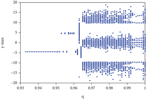
From the above dim(LE)s, it can be said that the Kaplan-Yorke dimension is decreased from 3.9975 to 3.6224, as the fractional order is increased from 0.857 to 1. Note that the Kaplan-York dimension determines the upper bound of the Hausdorff dimensions. In this study, the Hausdorff dimensions of the attractors corresponding to different fractional orders are nonintegers and system (5) has strange attractors with fractal structures. Moreover, in Table 1 and the Kaplan-Yorke dimensions calculated above, one can find that the significance of the hyperchaotic attractors decreases as the fractional order increases from 0.857 to 1. The loss of significance is described by decreasing the sum of the positive LEs in Table 1 and also by decreasing the dimensions as the fractional order increases from 0.857 to 1. The loss of significance is also observable from the bifurcation diagram of the fractional orders shown in Figure 1 in the next section.

5.2. Bifurcation for the Fractional Order η

The bifurcation diagram of the fractional order η is obtained by varying its value in the interval (0.857,1.00) with a time step of h = 0.001. The bifurcation diagram due to the variations of the order is illustrated in Figure 1. According to this figure, for values of η ∈ (0.933,0.953), the given system exhibits oscillation with stability and the system excites a chaotic behavior for fractional values η ≥ 0.953.

The simulation results corresponding to different fractional orders are portrayed in Figures 2–4 to verify the conclusion made in Figure 1.

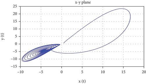
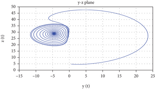
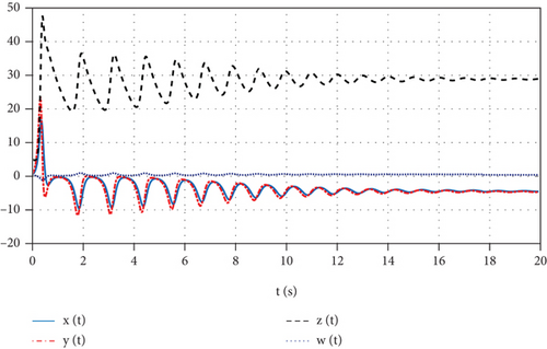
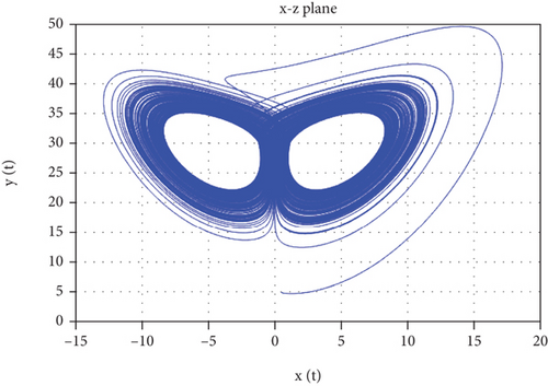
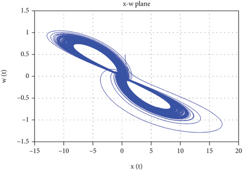
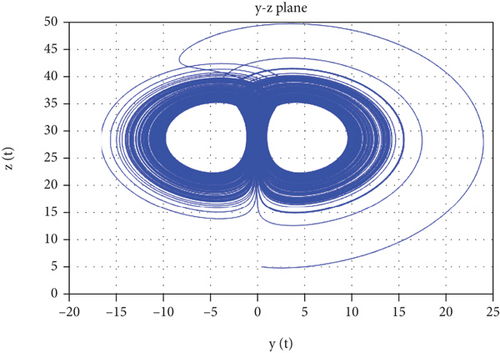
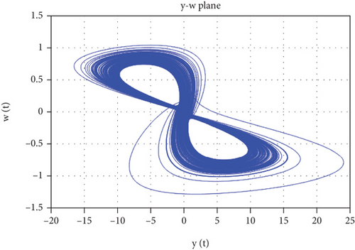
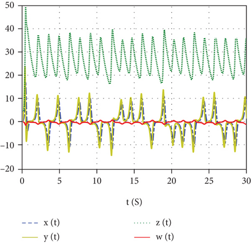
It can be seen in Figures 2(a)–2(c) that the system exhibits oscillation with stability for the fractional order η = 0.95 ∈ (0.933,0.953), which is in agreement with the conclusion in Figure 1. The time series solution of system (5) is shown for η = 0.95 in Figure 3, where the solution trajectories have the property of oscillation and stability as claimed from the bifurcation diagram shown in Figure 1. Moreover, Figures 4 and 5 characterize that system (5) exhibits a hyperchaotic behavior at η = 0.974 confirming what is predicted by the bifurcation diagram in Figure 1.

5.3. Bifurcation for Parameter r

To get the bifurcation diagram of parameter r of the hyperchaotic system (5), the fractional order used is η = 0.97 and k = 0.7, c = 4, a = 10, and r ∈ [29.5,30.5] with a time step of h = 0.001 and the initial value condition is y₀ = [0.5, 0.5, 5, 0.5]. The simulation is made to run for 100 s. The bifurcation graph due to the variation of r is illustrated in Figure 6.

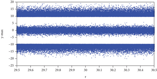
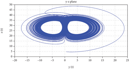
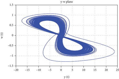
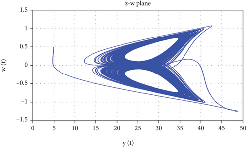
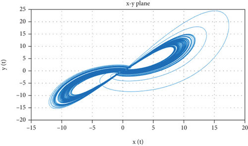
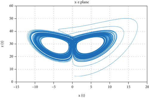
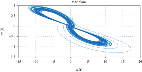
It can be inferred in Figure 6 that system (5) exhibits a hyperchaotic behavior for the parameters considered in the simulation for r ∈ [29.5,30.5]. The phase portraits of system (5) shown in Figures 7 and 8 for r = 29.6 and r = 30.4 verify the conclusion from the bifurcation diagram of Figure 6.

5.4. Bifurcation for Parameter c

For the bifurcation diagram of parameter c of the hyperchaotic system (5), the fractional order used is η = 0.974, k = 0.7, and a = 10 and the bifurcation parameter is made to vary in the interval [3.5, 4.5] with a time step of h = 0.001, with initial value condition y₀ = [0.5; 0.5; 5; 0.5], and the simulation is made to run for 100 s. The bifurcation diagram due to the variation of parameter c is illustrated in Figure 9.

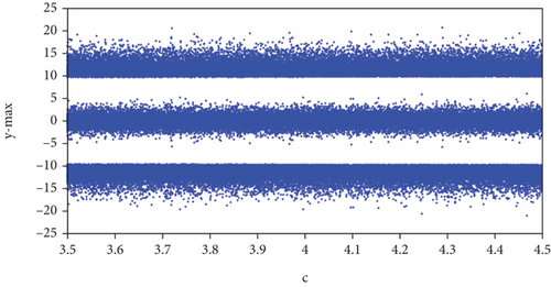
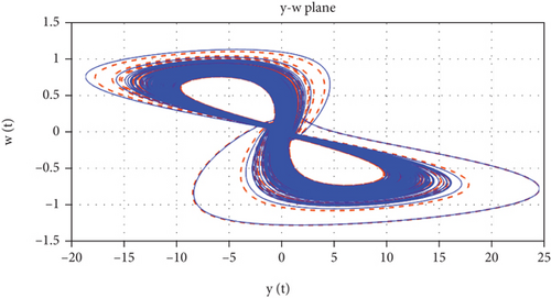
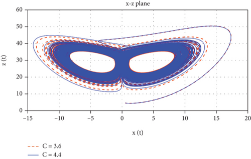
It is observable in Figure 5 that system (5) shows hyperchaotic dynamics for parameter c in [3.5, 4.5]. Moreover, the phase portraits of system (5) for c = 3.6 and 4.4 shown in Figure 10 verify the conclusion drawn in Figure 9.

5.5. Bifurcation for Parameter k

To obtain the bifurcation diagram due to parameter k of the hyperchaotic system (5), the fractional order used is η = 0.974. The values of the remaining parameters are k = 0.7 and a = 10, and the bifurcation parameter k is made to vary in the interval [0.5, 1] with a time step of h = 0.001. The initial value condition is y₀ = [0.5; 0.5; 5; 0.5] and the simulation is made to run for 100 s. The bifurcation graph due to the variation of k is illustrated in Figure 11.

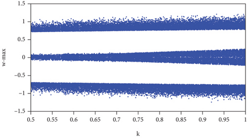
It is clear in Figure 11 that system (5) shows hyperchaotic dynamics for parameter k of the interval [0.5, 1], the given values of the parameters, and fractional orders. Moreover, the attractors of system (5) for values of parameter k in [0.5, 1] are approximately similar to the figures shown in Figure 10.

5.6. Bifurcation for Parameter a

To obtain the bifurcation diagram due to parameter a of the hyperchaotic system (5), the fractional derivative, the initial condition, the time, and the values of the remaining parameters are the same as those used in Section 5.5. The bifurcation diagram due to the variation of parameter a is illustrated in Figure 12.

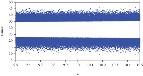
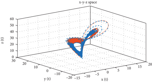
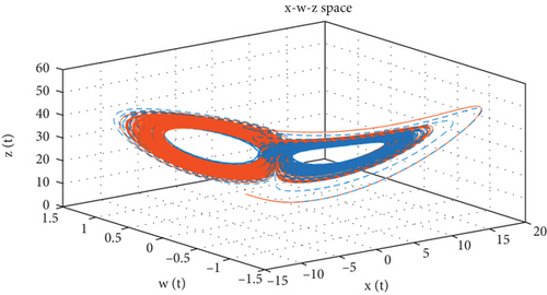
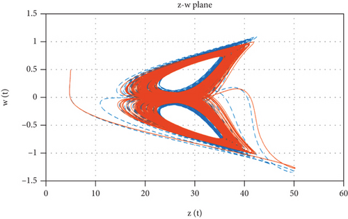
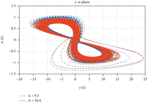
It is clear in Figure 12 that system (5) shows the hyperchaotic dynamics for parameter a in [9.5,10.5], the given parameters, and the fractional orders. Moreover, the attractors of system (5) for different values of a are shown in Figure 13, verifying the hyperchaotic nature of system (5).

6. Sensitivity to Initial Conditions

This section examines the effect of different initial values on the dynamics of the hyperchaotic system (5). Since sensitivity to initial conditions is one of the important properties of chaotic or hyperchaotic systems, it is necessary to examine this property for the LS system (5) using different initial conditions. In this study, to examine sensitivity to initial conditions, we used the parameter values indicated in (5) and η = 0.974. The initial condition considered is (x₀, 0.5,5, 0.5). The different values of x₀ are shown in Figure 14.

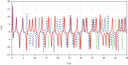
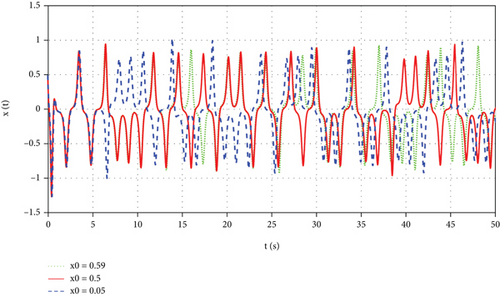
It can be observed in Figure 14 that all the trajectories coincided for about the first 5.1 seconds and they were divided into two for about 10.1 seconds. At about 15.1 seconds, they divided into three, diverging from each other. The values of x₀ of two trajectories that overlapped for the first 15.1 seconds are closer to each other than the value of x₀ of the third trajectory.

7. Synchronization of the Lorenz-Stenflo System

In this part of the study, we developed a master-slave system of the dynamic system (5). Firstly, two identical copies of system (5) are associated via a coupling function. Then, we performed a simulation of the coupled systems using different initial conditions. Finally, the error dynamics showed asymptotic stability and the phase portraits of the master and slave system showed a strong correlation.

It can be shown that all the real parts of the eigenvalues of H are negative. Thus, the Matignon criterion is satisfied; H is a Hermitian matrix.

To verify if the master and slave systems in equations (21) and (25) are correlated, the time series trajectories of the two systems, including the graphs of the dynamics of the error, are illustrated in Figures 15–19. The values of the parameters used are k = 0.7, r = 30, c = 4, and a = 10 together with the fractional order η = 0.978. Moreover, the initial value conditions used for the master and the slave system are y_0m = [0.5,0.5,5, 0.5] and y_0s = [5, 5, 5, 5], respectively.

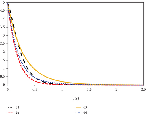
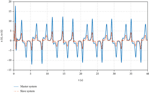
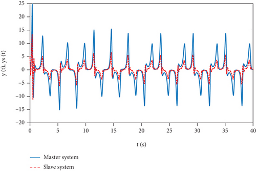
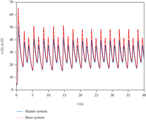
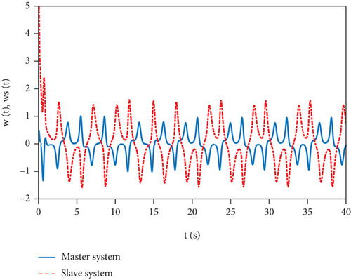
It can be observed in Figure 15 that there is a robust correlation between the master and slave systems because the error graphs converge to zero approximately in the first 2.5 seconds, as shown in Figure 15.

8. Conclusion

This research study implemented a qualitative analysis on the four-dimensional Lorenz-Stenflo mathematical model in the sense of the Caputo operator. The Matignon local stability criterion showed that the equilibrium points of the LS system are locally unstable, implying that the LS system led to hyperchaotic dynamical behavior. The scheme developed by Garrappa approximated the numerical solution, and the corresponding MATLAB code was used to obtain all the figures in the study. The authors believe that the qualitative analysis made in this manuscript, the displayed figures, and the synchronization systems developed have revealed complex dynamical behaviors of the Lorenz-Stenflo system that are not obtained earlier by other studies on the system. It is also worth mentioning that this study have been done by including other concepts of fractional derivatives and comparing the results to the results obtained due to the Caputo fractional derivative, to be treated in the future by the authors or interested researchers in the area.

Conflicts of Interest

The authors declare that they have no competing interests.

Authors’ Contributions

Chernet Tuge Deressa did the actualization, methodology, formal analysis, validation, investigation, and initial draft. Sina Etemad did the actualization, validation, methodology, formal analysis, investigation, and initial draft. Mohammed K. A. Kaabar did the actualization, methodology, formal analysis, validation, investigation, initial draft, and supervision of the original draft and editing. Shahram Rezapour did the actualization, validation, methodology, formal analysis, investigation, and initial draft. All authors read and approved the final version.