Volume 2022, Issue 1 4912859

Research Article

Open Access

[Retracted] The Mathematical Analysis of the New Fractional Order Ebola Model

Retraction(s) for this article

Faiz Muhammad Khan,

Faiz Muhammad Khan

Department of Mathematics and Statistics, University of Swat, Khyber Pakhtunkhawa, Pakistan uswat.edu.pk

Search for more papers by this author

Amjad Ali,

Amjad Ali

Department of Mathematics and Statistics, University of Swat, Khyber Pakhtunkhawa, Pakistan uswat.edu.pk

Search for more papers by this author

Ebenezer Bonyah,

Corresponding Author

Ebenezer Bonyah

[email protected]

orcid.org/0000-0001-8763-6164

Department of Mathematics Education, Akenten Appiah Menka University of Skills Training and Entrepreneurial Development, (Kumasi Campus), Ghana aamusted.edu.gh

Search for more papers by this author

Zia Ullah Khan,

Zia Ullah Khan

Department of Mathematics and Statistics, University of Swat, Khyber Pakhtunkhawa, Pakistan uswat.edu.pk

Search for more papers by this author

Faiz Muhammad Khan,

Faiz Muhammad Khan

Department of Mathematics and Statistics, University of Swat, Khyber Pakhtunkhawa, Pakistan uswat.edu.pk

Search for more papers by this author

Amjad Ali,

Amjad Ali

Department of Mathematics and Statistics, University of Swat, Khyber Pakhtunkhawa, Pakistan uswat.edu.pk

Search for more papers by this author

Ebenezer Bonyah,

Corresponding Author

Ebenezer Bonyah

[email protected]

orcid.org/0000-0001-8763-6164

Department of Mathematics Education, Akenten Appiah Menka University of Skills Training and Entrepreneurial Development, (Kumasi Campus), Ghana aamusted.edu.gh

Search for more papers by this author

Zia Ullah Khan,

Zia Ullah Khan

Department of Mathematics and Statistics, University of Swat, Khyber Pakhtunkhawa, Pakistan uswat.edu.pk

Search for more papers by this author

First published: 25 June 2022

https://doi.org/10.1155/2022/4912859

Citations: 4

Academic Editor: Mohammad Rahimi-Gorji

Share a link

Email
Wechat
Bluesky

Abstract

This research study focuses on the analytical behavior and numerical computation of the fractional order Ebola model. In this study we have calculated the conditions for the existence, uniqueness, and stability of the solution with the help of the fixed point results. In addition to this, we calculated the numerical solution of the fractional order smoke model with the help two-step fractional Adam’s Bashforth method using the Caputo’s fractional derivative of order μ. Furthermore, the results obtained for different orders of the fractional derivative μ have been shown graphically with the help of Matlab.

1. Introduction

The concept of fractional calculus (FC) was raised in seventeen century from famous correspondence between Leibniz and L’Hoptial. In the consequences of aforementioned correspondence, Leibniz wrote a letter to Guillaume de L’Hôpital that what will be the half order derivative of dependent variable y w.r.t x, i.e, d^1/2x/dy^1/2. In the response, he wrote that this will bear some useful consequence in near future. Later on, it was traced that fractional calculus was introduced by Abel in one of his papers, where the author discussed the idea of fractional-order derivatives (FOD), fractional-order integration (FOI), and the mutual inverse relationship between them [1]. In 1832, one of the greatest French mathematicians (of his era) Liouville presented the definitions for the fractional derivative and fractional integration named as Riemann-Liouville fractional derivative and integration [2]. Later, on in 1890, Heaviside practically used the fractional differential operator in electrical transmission line analysis circa [3]. Recently, the researchers of the 19th and 20th century have made their significant contributions to introduce new definitions of fractional differential and integral operators and in the study of the practical applications of FC [4].

In modern era, the uses of FC in various engineering problems have been raised [5–7] 2014). For instance, FC has various applications in different diffusion phenomenon including heat transfer, gaseous exchange, and water transfer through permeable materials [8–11]. Bagley and Torvik presented FC as an instrument for displaying tissue viscoelasticity during the 1980s (Uchaikin, 2013). Study of intricacy gives another view to a few genuine wonders which appeared to be odd, and during the most recent years, new strategies have been utilized to separate secret properties of complex frameworks [12]. Further, a variety of FC tools have been widely used in several complex phenomena [13–15]. In some circumstances, FC has been perceived for taking care of issues in viscoelasticity, electrochemistry, and dispersion [16–19]. A few analysts featured FC as a tool for examination of complex phenomenon by bringing the techniques of FC and its applications to a more extensive crowd [20, 21] .

The technique by which a real world problem is described in mathematical concepts or language is known as mathematical modeling [22]. Mathematical modeling of infectious diseases has been the main focus for the scientists and researchers over the last two decades. Mathematical modelers used to model the infectious diseases in the form of mathematical models consist of classical differential equations (CDEs). Recently, the researchers have diverted their focus to model the diseases in the form of fractional differential equations (FDEs) which has the potential to describe the real world phenomena more accurate and considered reliable as compared to the conventional derivatives. FDEs are global in nature, more realistic, and give great degree of freedom to modelers as compared to the CDEs. Modeling via FDEs has produced highly influential results in the investigation of transmission of the infectious diseases models [23, 24].

In the year 1976, a flare-up occurred in African nation of the Democratic Republic of Congo (DRC), which was then termed after the name of the lake “Ebola” flows near to the DRC. The infection has five sorts, four out of these five spread illnesses in people. The infection use to attack on the immune system which then cause internal bleeding and affect each organ of the individuals. This terrifying infection spread by contacting directly with the tainted individuals either via body fluids or direct skin contact. The infection can also be pass through connection with the creatures like monkeys, etc. Nonetheless, the infection cannot be transmit through air and food. Later on, in 2013, the infection arose in Guckduo and Guinea, where 28,616 casualties were reported, and out of these casualties, 11,310 lost their lives. Today, where the advanced world is confronting another pandemic flare-up as COVID-19, the investigation of such irresistible sicknesses is still a center of focus for the researchers [25].

2. Model Formulation

In this section of the article, we have presented the formulation of the model, which we will be studying in this paper. For this, we have considered a population and divided it into five different compartments with some assumptions. The assumptions considered for the formulation of the model are stated below

(i)
: the first class of the model has been named as susceptible class. This class contains individuals who have no symptoms or any infection of the disease but can be attacked by the virus
(ii)
: the second class of the population has been named as exposed class. This class contains individuals who have been attacked by the virus but not yet shown the symptoms of the infection or not yet infectious
(iii)
: this is the third class of the population containing individuals who have been attacked by the virus and are being able to transfer the disease to not yet attacked individuals of the populations
(iv)
: this class has been named as vaccinated class containing those individuals of the susceptible class who have been vaccinated against the virus
(v)
ℝ: this class is the recovered class which contains those individuals who have survived the disease

The transition or transfer among the compartments has been considered in the following manner

(i)
: an individual of the population move to the population through the rate τ₁
(ii)
: an individual of the class joins the class with the rate β after getting infectious
(iii)
: the given parameter is used for the rate of the vaccination which transfer an individual from to
(iv)
: the rate of transfer of the individuals from to ℝ after surviving the disease
(1)

And the corresponding fractional form of the system (1) is

(2)

The paper has been organized as follows: the first section of the paper contains introduction. The second section has been restricted to the formulation of the model, while the third section has been devoted to the preliminaries. The fourth section of the paper contains the existence and uniqueness of the solution of the model. The fifth section of the paper includes the stability of the solution, while the sixth section contains qualitative study where we formulated the disease free, disease endemic, and basic reproduction number R₀ and then test the stability of the R₀ locally with the help of theorems. In the seventh section, we have formulated the numerical solution of the model via Adam’s Bashforth scheme, and the eighth section contains the numerical simulation of the results obtained in the section seventh. At last, we have concluded our work in the conclusion section.

3. Preliminaries

In this section of the present article, we provide some basic definitions, theorems, and results that will be used and fruitful in understanding the rest of the article.

Definition 1. (see [26].)The Caputo’s fractional differential operator of any arbitrary order μ > 0 is defined as

(3)

Lemma 2. (see [27].)“The following result holds for fractional differential equations

(4)

for arbitrary α_i ∈ R, i = 0, 1, 2, 3, ⋯, m − 1, where m = [μ] + 1 and [μ] symbolizes the integer part of μ”.

Lemma 3. (see [28].)Let θ ∈ ACⁿ[0, T], μ > 0, and n = [μ], then the following result holds

(5)

Lemma 4. (see [28].)In view of Lemma 3, the solution of , n − 1 < μ < n is given by

(6)

where c_j ∈ R.

Definition 5. (see [26].)Suppose we have Caputo’s fractional differential equation of order μ

(7)

then the solution is given as

(8)

where represent the remainder term. For the study of convergence and uniqueness of the solution of the scheme, we refer to ([26]).

Theorem 6. (see [29].)“Let X be a Banach space and is compact and continuous, if the set,

(9)

is bounded, then has a unique fixed point.”

4. Existence of the Solution

In this section of the paper, we construct the conditions for the existence and uniqueness of the solution, and to get the desired results, we construct the following function.

(10)

Suppose that the considered space

be a Banach space with norm

(11)

where

(12)

With the help of (12), the system (1) can be written in as

(13)

By Lemma 2, equation (13) converts into the following form

(14)

To prove the existence of the solution, we make the following assumptions:

(P1)∃ constants

∋

(15)

(P2)∃L_∗ > 0, ∋ for each

(16)

And let

be an operator as

(17)

Theorem 7. When the assumptions (P1) and (P2) are true, it verifies that the problem (13) has at least of one fixed point which also implies that the problem of our study has also at least one solution.

Proof. Furthermore we proceed as.

Step 1. First, we have to show that is continuous. To acquire the results, we suppose that is continuous for j = 1, 2, 3, 4, 5, 6. Which implies that is also continuous. Assume θ_n.θ ∈ X∋θ_n⟶θ, we must have .

For this, we consider

(18)

As is continuous, therefore , yields that is continuous.

Step 2. Now, to prove that is bounded for any , we make of the supposition that satisfies the growth condition:

(19)

Here, we assume a , the subset of with the property of boundedness, and we need to prove that is also bounded. To reach our destination, we assume that for any , now as is bounded, so ∃K_q ≥ 0∋

(20)

Further, for any by using the growth condition, we have

(21)

Therefore, is bounded.

Step 3. Here, we attempt to prove that the operator we defined is equicontinuous, for this we assume that t₂ ≤ t₁ ∈ J = [0, T], then

(22)

By taking advantage of Arzelà-Ascoli theorem, we can say that is relative compact.

Step 4. In this step, we need to prove that the set defined below is bounded

(23)

To prove this, we suppose that θ ∈ E, ∋ for each t ∈ J, where J = [0, T] we have

(24)

From here, we can claim that the set defined above is bounded. By using Schaefer’s FPT, the operator we defined, i.e., has atleast one fixed point, and hence, the model we studied in this paper has at least one solution.

Theorem 8. The problem (13) is unique solution, if .

Proof. Let , then

(25)

Hence, we can say that the fixed point is unique, and therefore, our solution is unique.

5. Stability Results

To prove that the solution of the considered model is stable, we use the concept of Ulam and Ulam Hyer stability. To get the desired results we proceed as

Assume

be an operator which satisfy

(26)

Definition 9. (see [27].)Equation (26) has UH-stability, if for ς₁ > 0 and assume any solution for the inequality given by

(27)

and the unique solution

for (25) with

, such that

(28)

Definition 5.2. “If ∃ϑ ∈ C(R, R) with ϑ(0) = 0, ” for unique result and any solution of equation (26) ∋

(29)

then equation (26) has GUH-stability.

Remark 10. (see [27].)“If ∋, then satisfies (27) if

(i)

(ii) ”

For further analysis, we suppose that the following is the solution of the perturbed problem of (13)

(30)

Lemma 11. The result stated below holds true for equation (30),

(31)

Theorem 12. By making use of Lemma 11, the solution of the problem (13) is UH-stable as well as GUH-stable, if T^μL_ω/Γ(μ + 1) < 1.

Proof. Assume be any and unique solutions, respectively, problem (13), then

(32)

From here, we claim that the solution of (13) is UH and GUH stability if

(33)

Such that Y(0) = 0.

Definition 13. The UHR-Stability of (26) is ensured for g^∗ ∈ C([0, T], R), if for ς₁ > 0 and assume θ ∈ X be any solution of the inequality expressed by

(34)

∃ a unique solution of (26) with ∋

(35)

Definition 14. (see [27].)“For g^∗ ∈ C[0, T], R], if ∃ and for ς₁ > 0, consider that θ be any solution of (34) and be any solution of (26) ∋

(36)

then equation (26) is generalized UHR stable.”

Remark 15. If ∃, then for (27) holds, if

(i)
(ii)

Lemma 16. The stated result below holds true for (30)

(37)

Proof. The proof has been left for the readers.

Theorem 17. With the help of Lemma 16, our solution is Ulam and Generalized Ulam stable if T^μL_θ/Γμ + 1 < 1.

Proof. . Assume be two solutions such that θ is any and any and is the unique solution of our problem, then

(38)

Hence, the solution possesses both type of the stabilities.

6. Qualitative Study

In this section of the article, we present disease free equilibrium, disease endemic equilibrium, the basic reproduction number R₀, and the local assymptotical stability of the R₀. To proceed, we first find the disease free equilibrium and disease endemic equilibrium of the model. The disease free equilibrium is given as S⁰ = (Λ/d₀ + ψ, 0, 0, 0, 0), while the endemic equilibrium is given below.

6.1. Endemic Equilibrium

The endemic equilibrium of the model is given as

(39)

6.2. The Basic Reproduction Number

To find R₀, we construct two vectors such as

(40)

(41)

Now, we present the Jacobian of both the matrix, i.e.,

(42)

(43)

with

(44)

Now, to find the next generation matrix (NGM), we find the product of

and

, i.e.,

(45)

Clearly, the eigen values are (say) λ₁ and λ₂ which are given as and . Therefore, the basic reproduction number R₀ = max(λ₁, λ₂).

Theorem 18. The basic reproduction number R₀ is locally assymptotically stable at the disease free equilibrium point that is stable if R₀ < 1.

Proof. For this purpose, we construct the following Jacobian.

(46)

Now, let the eigen values are (say) λ₁, λ₂, λ₃, λ₄, λ₅. Clearly λ₁ = λ₂ = −d₀, λ₃ = τS⁰ − (d₀ + d₁ + κ), λ₄ = −(d₀ + ψ), and . From λ₃, we have , and from λ₅, we have . Therefore, R₀ = max(λ₃, λ₅) < 1 and hence is locally assymptotically stable at the disease free equilibrium point.

Theorem 6.2. The basic reproduction number R₀ is locally assymptotically stable at the endemic equilibrium point if R₀ > 1.

Proof. The proof of this result can be obtained on the same manner as the proof in [30].

7. Numerical Solution

This section of the article is devoted to the numerical solution of the considered model. For this, we will use the well-known two-step fractional order Adam’s Bashforth method. The considered model is given as

(47)

To obtain the desired results, we apply the fundamental theorem of fractional calculus to system (3) gives

(48)

The unknown terms

are given below. Now, for t = t_n+1, we get

(49)

For t = t_n, we get the following

(50)

, and ℝ(t_n+1) − ℝ(t_n) in (49) and (50), we obtain

(51)

where

(52)

(53)

By approximating

, and

with the help of Lagrange’s polynomials and the plugging back in (51), we get the following solution

(54)

where

(55)

And , , , , and are the remainder’s terms.

8. Numerical Simulation

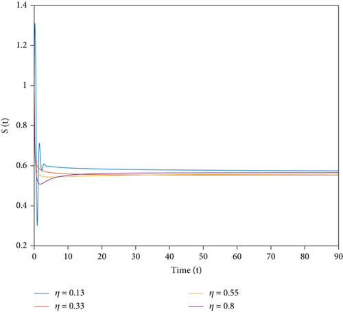
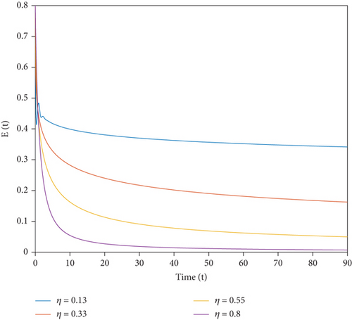
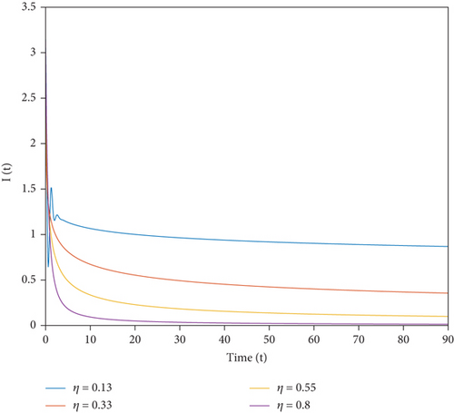
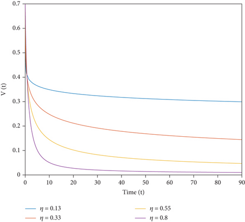
In this section of the article, we present the graphical results of the solution obtained in (54). For this purpose we have simulated the results via Matlab by assigning the values given in (Table 1) to the parameters and classes of the model. The graphical results are shown in the following.

Table 1. The physical interpretation and numerical values of the parameters.

Parameters	Physical description	Numerical value	Source
Λ	The birth rate	0.4	Assumed
d₀	Natural death rate	0.7	Assumed
d₁	Disease death rate in	0.075	Assumed
d₂	Disease death rate in	0.35	Assumed
τ	The contact rate of and	0.14280	Assumed
κ	The transference rate from to	0.048	Assumed
β	The contact rate of and	0.35	Assumed
ξ	Recovery rate	0.53	Assumed
ψ	Vaccination rate	0.00493	Assumed

9. Discussion

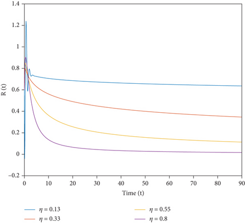
Figure 1 describes the dynamics of susceptible population for different values of the order of fractional derivatives. Each curve tends to the equilibrium solution irrespective of the value of μ. As we increase the value of μ, the rate of convergence to the stated equilibrium increases. Figure 2 represents the behavior of E(t) along the time direction, and the figure shows that for describing the slow evolution of disease, one might assume small values of μ. Infection from the community could be rapidly eliminated by increasing the order of the derivative as shown in Figure 3. A similar conclusion could be drawn from Figures 4 and 5, i.e., to capture the realistic scenario of slowly spreading diseases, one must consider the tools of fractional order derivative while modeling such epidemics.

Details are in the caption following the image — **Figure 1**
Open in figure viewer PowerPoint

The behavior of susceptible population.

10. Conclusion

In this paper, we have studied the fractional order Ebola model containing Caputo’s fractional derivative of order μ. The paper contains the study related to the existence of the solution performed by using theorems of fixed point theory for the existence of fixed point. In addition, we have proved that the solution of the system is unique as well as Ulam stable. Apart from this, we have find the numerical solution of the studied model with the help of two-point fractional order Adam’s Bashforth method presented for the approximation of the fractional differential equations containing the Caputo’s fractional derivative. In addition, we have visualized the results graphically with the help of Matlab. At last, we have discussed the dynamical behavior of the obtained solution for all classes of the said model.

Conflicts of Interest

The authors declare that they have no conflicts of interest.

Open Research

Data Availability

The data will be for public after the publication.

References

1 Podlubny I., Magin R. L., and Trymorush I., Niels Henrik Abel and the birth of fractional calculus, Analysis. (2017) 20, no. 5, 1068–1075, https://doi.org/10.1515/fca-2017-0057, 2-s2.0-85034090676.
10.1515/fca-2017-0057
Web of Science® Google Scholar
2 Dugowson S., Les differetielles metaphysiquos: historie et philosophie de la generalisation de I’ order de la derivation par, 1994, Paris.
Google Scholar
3 Ross B., The development of fractional calculus 1695-1900, Historia Mathematica. (1977) 4, no. 1, 75–89, https://doi.org/10.1016/0315-0860(77)90039-8, 2-s2.0-23644455602.
10.1016/0315-0860(77)90039-8
Google Scholar
4 Valerio D., Machado J. T., and Kiryakova V., Some pioneers of the applications of fractional calculus, Fractional Calculus and Applied Analysis. (2014) 17, no. 2, 552–578, https://doi.org/10.2478/s13540-014-0185-1, 2-s2.0-84896939823.
10.2478/s13540-014-0185-1
Web of Science® Google Scholar
5 West B. J., Fractional Calculus View of Complexity: Tomorrow’s Science, 2015, 1st edition, CRC Press.
Google Scholar
6 Nighmanullin R. R., Giniatullin R. A., and Skorinkin A. I., Membrane current series monitoring: essential reduction of data points to finite number of stable parameters, Frontiers in Computational Neuroscience. (2014) 8, https://doi.org/10.3389/fncom.2014.00120, 2-s2.0-84907573940.
10.3389/fncom.2014.00120
Web of Science® Google Scholar
7 Sharma A., Namsani S., and Singh J. K., Molecular simulation of shale gas absorption and diffusion in inorganic nanopores, Molecular Simulation. (2014) 415, no. 5-6, 414–422, https://doi.org/10.1080/08927022.2014.968850, 2-s2.0-84922676485.
10.1080/08927022.2014.968850
Google Scholar
8 Metzler R., Jeon J. H., Cherstvy A. G., and Barkai E., Anomalous diffusion models and their properties: non-stationarity, non-ergodicity, and ageing at the centenary of single particle tracking, Physical Chemistry Chemical Physics. (2014) 16, no. 44, 24128–24164, https://doi.org/10.1039/C4CP03465A, 2-s2.0-84908129836, 25297814.
10.1039/C4CP03465A
CAS PubMed Web of Science® Google Scholar
9 Garappa R., Grunwald-Letnikov operators for fractional relaxation in Havriliak-Negami models, Communications in Nun linear Science and Numerical SImulation. (2016) 38, 178–191, https://doi.org/10.1016/j.cnsns.2016.02.015, 2-s2.0-84960452510.
10.1016/j.cnsns.2016.02.015
Web of Science® Google Scholar
10 Yang X., Chen W., Xiao R., and Ling L., A fractional model for time-variant non-Newtonian flow, Thermal Science. (2017) 21, no. 1 Part A, https://doi.org/10.2298/TSCI160426245Y, 2-s2.0-85015685601.
10.2298/TSCI160426245Y
Web of Science® Google Scholar
11 Uchaikin V., Fractional derivatives for physicists and engineers. Volume I background and theory volume II applications (nonlinear physical science) (2013th ed.), 2013, Springer.
Google Scholar
12 Benson D. A., Wheatcraft S. W., and Meerschaert M. M., The fractional-order governing equation of Lévy motion, Water Resources Research. (2000) 36, no. 6, 1413–1423, https://doi.org/10.1029/2000WR900032, 2-s2.0-0034113992.
10.1029/2000WR900032
Web of Science® Google Scholar
13 Feliu-Talegon D., San-Millan A., and Feliu-Batlle V., Fractional-order integral resonant control of collocated smart structures, Control Engineering Practice. (2016) 56, 210–223, https://doi.org/10.1016/j.conengprac.2016.07.016, 2-s2.0-84991203999.
10.1016/j.conengprac.2016.07.016
Web of Science® Google Scholar
14 Atangana A. and Araz S. I., Mathematical model of COVID-19 spread in Turkey and South Africa: theory, methods, and applications, Adv. Difference Equ.(2020) 2020, no. 1, https://doi.org/10.1186/s13662-020-03095-w, 33391372.
10.1186/s13662-020-03095-w
PubMed Web of Science® Google Scholar
15 Araz S. İ., Analysis of a COVID-19 model: optimal control, stability and simulations, Alexandria Engineering Journal. (2021) 60, no. 1, 647–658, https://doi.org/10.1016/j.aej.2020.09.058.
10.1016/j.aej.2020.09.058
Web of Science® Google Scholar
16 Wu G., Baleanu D., and Zeng S.–. D., Finite-time stability of discrete fractional delay systems: Gronwall inequality and stability criterion, Communications in Nonlinear Sciences and Numerical SImulation. (2018) 57, 299–308, https://doi.org/10.1016/j.cnsns.2017.09.001, 2-s2.0-85031123110.
10.1016/j.cnsns.2017.09.001
Web of Science® Google Scholar
17 Burke K. and Mather P. T., Soft shape memory in main-chain liquid crystalline elastomers, Journal of Materials Chemistry. (2010) 20, no. 17, https://doi.org/10.1039/b924050k, 2-s2.0-77953046667.
10.1039/b924050k
Google Scholar
18 Lendlein A. and Langer R., Biodegradable, elastic shape-memory polymers for potential biomedical applications, Science. (2002) 296, no. 5573, 1673–1676, https://doi.org/10.1126/science.1066102, 2-s2.0-0037204998, 11976407.
10.1126/science.1066102
CAS PubMed Web of Science® Google Scholar
19 Li C. and Zeng F., Numerical Methods for Fractional Calculus, 2020, 1st edition, Chapman and Hall/CRC.
Google Scholar
20 Lenzi E., Zola R. S., Rossato R., Ribeiro H. V., Vieira D. S., and Evangelista L. R., Asymptotic behaviors of the Poisson-Nernst-Planck model, generalizations and best adjust of experimental data, Electrochemia Acta. (2017) 226, 40–45, https://doi.org/10.1016/j.electacta.2016.12.075, 2-s2.0-85008235303.
10.1016/j.electacta.2016.12.075
CAS Web of Science® Google Scholar
21 Wang X., Qi H., Yu B., Xiong Z., and Xu H., Analytical and numerical study of electroosmotic slip flows of fractional second grade fluids, Communications in nonlinear sciences and numerical simulation. (2017) 50, 77–87, https://doi.org/10.1016/j.cnsns.2017.02.019, 2-s2.0-85014503465.
10.1016/j.cnsns.2017.02.019
Web of Science® Google Scholar
22 Zill D. G., A First Course in Differential Equations with Modeling Application, 2017, 11th edition, Cengage Learning.
Google Scholar
23 Atangana A., Fractional operators and their applications, Fractional Operators with Constant and Variable order with application to Geo-Hydrology, 2018, Elsevier, 79–112, https://doi.org/10.1016/B978-0-12-809670-3.00005-9.
10.1016/B978-0-12-809670-3.00005-9
Google Scholar
24 Liu P., Munir T., Cui T., Din A., Wu P., School of Statistics and Mathematics, Guangdong University of Finance and Economics, Big data and Educational Statistics Application Laboratory Guangzhou 510320, China, School of Statistics and Mathematics, Guangdong University of Finance and Economics, Guangzhou 510320, China, Abdus Salam School of Mathematical Sciences GC University Lahore, 54600 Pakistan, School of Economics, Guangdong University of Finance and Economics, Guangzhou 510320, China, Department of Mathematics Sun Yat-sen University, Guangzhou 510275, China, and School of Data Sciences, Zhejiang University of Finance & Economics, Hangzhou 310018, China, Mathematical assessment of the dynamics of the tobacco smoking model: an application of fractional theory, AIMS Mathematics. (2022) 7, no. 4, 7143–7165, https://doi.org/10.3934/math.2022398.
10.3934/math.2022398
Web of Science® Google Scholar
25 Tahir M., Zaman G., Shah A., Muhammad S., Hussain S. A., and Ishaq M., The stability analysis and control transmission of mathematical model for Ebola virus, Open Journal of Mathematical Analysis. (2019) 3, no. 2, 91–102, https://doi.org/10.30538/psrp-oma2019.0042.
10.30538/psrp-oma2019.0042
Google Scholar
26 Atangana A. and Owlabi K. M., New numerical approach for fractional differential equations, Mathematical Modelling of Natural Phenomena. (2018) 13, no. 1, https://doi.org/10.1051/mmnp/2018010, 2-s2.0-85045204146.
10.1051/mmnp/2018010
Web of Science® Google Scholar
27 Khan Z. U., Ali A., Khan F. M., and Shah K., Existence theory and numerical simulation of ebola model corresponding to nonlocal fractional order derivative, Arab Journal of Basic and Applied Sciences. (2020) 27, no. 1, https://doi.org/10.1080/25765299.2020.1826668.
10.1080/25765299.2020.1826668
PubMed Google Scholar
28 Ali A., Existence Theory & Numerical Solution of Boundary Value Problems for Fractional Differential Equations[PhD Desertation] UoM, 2017.
Google Scholar
29 Granas A. and Dugundji J., Fixed Point Theory, 2003, Springer-Verlag, New York, https://doi.org/10.1007/978-0-387-21593-8.
10.1007/978-0-387-21593-8
Web of Science® Google Scholar
30 Khan F. M., Ali A., Khan Z. U., Alharthi M. R., and Abdel-Aty A. H., Qualitative and quantitative study of Zika virus epidemic model under Caputo’s fractional differential operator, Physica Scripta. (2021) 96, no. 12, https://doi.org/10.2021/1402-4896/ac259e.
10.2021/1402-4896/ac259e
Web of Science® Google Scholar

Citing Literature

All articles

[Retracted] The Mathematical Analysis of the New Fractional Order Ebola Model

Retraction(s) for this article

Retracted: The Mathematical Analysis of the New Fractional Order Ebola Model

Abstract

1. Introduction

2. Model Formulation

3. Preliminaries

4. Existence of the Solution

5. Stability Results

6. Qualitative Study

6.1. Endemic Equilibrium

6.2. The Basic Reproduction Number

7. Numerical Solution

8. Numerical Simulation

9. Discussion

10. Conclusion

Conflicts of Interest

Open Research

Data Availability

References

Citing Literature

Figures

References

Information

About Wiley Online Library

Help & Support

Opportunities

Connect with Wiley

[Retracted] The Mathematical Analysis of the New Fractional Order Ebola Model

Retraction(s) for this article

Retracted: The Mathematical Analysis of the New Fractional Order Ebola Model

Abstract

1. Introduction

2. Model Formulation

3. Preliminaries

4. Existence of the Solution

5. Stability Results

6. Qualitative Study

6.1. Endemic Equilibrium

6.2. The Basic Reproduction Number

7. Numerical Solution

8. Numerical Simulation

9. Discussion

10. Conclusion

Conflicts of Interest

Open Research

Data Availability

References

Citing Literature

Figures

References

Related

Information