Volume 2022, Issue 1 4557844

Research Article

Open Access

Analysis of Two-Level Mesh Method for Partial Integro-Differential Equation

Quan Tang,

Quan Tang

School of Mathematical Sciences, Xinjiang Normal University, Urumqi 800017, China xjnu.edu.cn

Search for more papers by this author

Ziyang Luo,

Ziyang Luo

School of Mathematical Sciences, Xinjiang Normal University, Urumqi 800017, China xjnu.edu.cn

Search for more papers by this author

Xindong Zhang,

Corresponding Author

Xindong Zhang

[email protected]

orcid.org/0000-0002-9879-8019

School of Mathematical Sciences, Xinjiang Normal University, Urumqi 800017, China xjnu.edu.cn

Search for more papers by this author

Juan Liu,

Juan Liu

College of Big Data Statistics, Guizhou University of Finance and Economics, Guiyang 550025, China gzife.edu.cn

Search for more papers by this author

Quan Tang,

Quan Tang

School of Mathematical Sciences, Xinjiang Normal University, Urumqi 800017, China xjnu.edu.cn

Search for more papers by this author

Ziyang Luo,

Ziyang Luo

School of Mathematical Sciences, Xinjiang Normal University, Urumqi 800017, China xjnu.edu.cn

Search for more papers by this author

Xindong Zhang,

Corresponding Author

Xindong Zhang

[email protected]

orcid.org/0000-0002-9879-8019

School of Mathematical Sciences, Xinjiang Normal University, Urumqi 800017, China xjnu.edu.cn

Search for more papers by this author

Juan Liu,

Juan Liu

College of Big Data Statistics, Guizhou University of Finance and Economics, Guiyang 550025, China gzife.edu.cn

Search for more papers by this author

First published: 13 July 2022

https://doi.org/10.1155/2022/4557844

Academic Editor: Feliz Minhos

Share a link

Email
Wechat
Bluesky

Abstract

In this paper, we present two-level mesh scheme to solve partial integro-differential equation. The proposed method is based on a finite difference method. For the first step, we use finite difference method in time and global radial basis function (RBF) finite difference (FD) in space. For the second step, we use the finite difference method to solve the proposed problem. This two-level mesh scheme is obtained by combining the radial basis function with finite difference. We prove the stability and convergence of scheme and show that the convergence order is O(τ² + h²), where τ and h are the time step size and space step size, respectively. The results of numerical examples are compared with analytical solutions to show the efficiency of proposed scheme. The numerical results are in good agreement with theoretical ones.

1. Introduction

For partial integro-differential equation,

(1)

where A and B are linear or nonlinear operators, the kernel κ(t, s) is the weakly singular function, and f(x, t) is given function. T is the terminal time, and Ω denotes a bounded domain with boundary Γ, where Ω ⊂ ℝ^d with d = 1, 2, 3.

This kind partial integro-differential equation is indicated by Volterra [1]; the new results of Volterra partial integro-differential equation can be found in [2, 3]. The problem Equation (1) can be found in the model of heat flow in a conducting materials with memory [4–7] and in viscoelastic mechanics [8–10].

In this paper, our particular concern is to obtain stability and convergence results for finite difference scheme and then use two-level mesh method to solve the following partial integro-differential equation. The following equation can be obtained by Equation (1), as Au(x, t) = Δu(x, t) = ∂²u(x, t)/∂x², Bu(x, s) = ∂²u(x, s)/∂x², and κ(t, s) = (t − s)^β−1.

(2)

where 0 < β < 1, f(x, t), and φ(x) are known functions. Throughout this paper, we assume that Equation (2) has a unique solution in [0, L] × [0, T] and suppose that ∂⁴u(x, t)/∂x⁴ and ∂³u(x, t)/∂t³ are continuous in [0, L] × [0, T].

Some attention has been paid to numerical methods of Equation (2), such as spectral collocation approximation by Kim and Choi [11], orthogonal spline collocation by Yan and Fairweather [12], alternating direction implicit difference scheme by Qiao and Xu [13], finite difference scheme by Tang [14], and compact difference scheme by Luo et al. [15]. If A is nonlinear operator, the numerical investigations for Equation (1) have been studied by several authors; one can refer to [16–18]. If we replace ∂u(x, t)/∂t with a fractional differential operator, then the fractional integro-differential equations can be obtained. The numerical solutions of fractional integro-differential equations have been studied by several authors; one can refer to [19–23].

Radial basis function, as a meshless method, has advantage of the ability to handle scattered node layouts and has the characteristics of simple implementation and high precision. The mainly purpose of this paper is to construct a numerical scheme using RBF and FD to solve partial integro-differential equation. In recent years, there are many researchers that studied the meshless method for solving partial differential equations. For example, Oruç developed a meshless approach based on radial basis function-finite difference (RBF-FD) method for solving one-dimensional, two-dimensional, and three-dimensional Schrödinger system [24, 25], two-dimensional fractional cable equation [26], and wave equations [27, 28]. Nikan and Avazzadeh [29] constructed an improved localized radial basis-pseudospectral numerical method for solving fractional reaction-subdiffusion equation.

This paper is outlined as follows. In Section 2, we introduce some notations and lemma and propose a two-level mesh discrete scheme based on finite difference. In Section 3, we discuss the stability and error estimation of the constructed discrete scheme. In Section 4, we consider the two-level algorithm which will be used in practical calculation. For more details on a two-level method, see [30, 31]. In Section 5, the results of numerical experiments are compared with exact solution to confirm the efficiency of the proposed discrete scheme. Finally, the conclusion and future studies are given for this paper in Section 6.

2. Construction of Numerical Scheme

In this section, we mainly consider the construction of discrete scheme. The following notations will be used in this section and others. Let M and N be positive integers. Let x_j≔jh with j = 0, 1, ⋯, M and t_k≔kτ with k = 0, 1, ⋯, N, where h≔L/M and τ≔T/N are the spatial and temporal step sizes, respectively. Let V_h = {V|V = (V₀, V₁, ⋯, V_M)} be the grid function space. For any functions V, W ∈ V_h, we define the following notations:

(3)

Throughout this paper, the values of C in different places are allowed to be different. Lemma 1 will be used in the construction of numerical scheme.

Lemma 1 (see [32].)If g(t) ∈ C²[0, T], then,

(4)

where C is a constant depending only on β(0 < β < 1) and

(5)

Now, we will consider the terms of Equation (2) one by one, and construct the discrete scheme of Equation (2).

For the term ∂u(x, t)/∂t in the left hand side of Equation (2), by the Taylor expansion, we obtain that

(6)

For the first term ∂²u(x, t)/∂x² in the right hand side of Equation (2), by the Taylor expansion, we obtain that

(7)

For the second term

in the right hand side of Equation (2), by Lemma 1 and the Taylor expansion, we obtain that

(8)

For j = 0, 1, ⋯, M and k = 0, 1, ⋯, N, we use

and

to denote the exact solutions of u(x_j, t_k) and f(x_j, t_k), respectively. If substituting Equations (6), (7), and (8) into Equation (2), then, we have

(9)

where

and C is a positive constant with independent τ and h.

Let

and

be the numerical approximation solutions of u(x_j, t₋₁) and u(x_j, t_k), respectively. Omitting small term

in Equation (9), the discrete scheme of Equation (2) can be obtained as follows:

(10)

3. Stability and Convergence

In this section, our purpose is to investigate the stability and convergence of the discrete scheme Equation (10). Some lemmas will be given for the proof of the main results. For convenience, we omit the subscript j from this section.

Lemma 2 (see [16].)If V, W ∈ V_h, then

Lemma 3 (see [16].)If V, W ∈ V_h, then

Lemma 4. (see [33].)Let λ_i,k be defined as in (5). For 0 < β < 1 and 0 ≤ i ≤ k, each of the following holds.

(i)
λ_i,k > 0, in particular, 0 < λ_0,k < τ^β/(β + 1), 1 ≤ k ≤ N
(ii)

Let u_t≔∂u(x, t)/∂t, in particular, denote u(x, t₋₁) ≈ u⁻¹ = u(x, 0) − τu_t(x, 0), where t₋₁ = −τ. By Taylor expansion, Lemma 5 can be obtained easily. We omit the proof of this lemma.

Lemma 5. Let and ε⁻¹ = u(x, t₋₁) − u⁻¹. Assume that u_t ∈ C²(0, T); then |ε⁻¹| ≤ Cτ².

Theorem 6 is about stability of discrete scheme Equation (10).

Theorem 6. Let U^k be the numerical solution of Equation (10) with the given initial and boundary conditions; if τ ≤ C₁h², then,

(11)

where C₁ and C are positive constants.

Proof. Since u⁻¹ = u⁰ − τu_t, by the assumption that u_t is continuous in the given domains, we get that ‖u⁻¹‖ ≤ C(‖u⁰‖ + τ‖u_t‖) < ∞, where C is a positive constant.

By Equation (10), we get that

(12)

Multiplying both sides of Equation (12) by U^k and integrating on [0, L], we obtain that

(13)

By Lemma 2, we have . Thus, Equation (13) can be rewritten as

(14)

In the following, we will use mathematical induction to prove our theorem. For k = 1, by Equation (14) and λ_0,1 = τ^β/(β + 1), we get that

(15)

Using Cauchy-Schwarz inequality and Lemma 3, we get

(16)

i.e.,

(17)

Assuming that holds for k ≤ N − 1, we want to prove that

(18)

Similarly, for k = N, by Equation (14), we get that

(19)

Using Cauchy-Schwarz inequality, Lemma 3, Lemma 4 and (τ/h²) ≤ C₁, we get

(20)

i.e.,

(21)

This proves the theorem.

In order to establish the convergence of proposed method, the following notations and results are needed. For V⁰ ∈ V_h, let Φ⁰ = u⁰ − V⁰, Ψ⁰ = V⁰ − U⁰,

, and

; then we obtain that

(22)

The convergence theorem and an error bound will been given for discrete scheme Equation (10) as follows.

Theorem 7. Let u^k be the exact solution of Equation (2) and U^k be the numerical solution of Equation (10). Letting e^k = u^k − U^k, then, for τ ≤ C₁h² and the given initial and boundary conditions, the following holds:

(23)

where C₁ and C are positive constants.

Proof. Subtracting Equation(10) from Equation(9), we obtain

(24)

where e⁰ = 0 and e⁻¹ will be discussed in the following.

Multiplying both sides of Equation (25) by e^k and integrating on [0, L], by Lemmas 1, 2, and 4, we obtain

(25)

Using Cauchy-Schwarz inequality, Lemma 3 and (τ/h²) ≤ C₁, we have

(26)

i.e.,

(27)

In order to prove this theorem, we first prove that ‖e⁻¹‖ = ‖u(x, t₋₁) − U⁻¹‖ ≤ C(τ² + h²). By Lemma 5 and (22), we get that

(28)

Next, we use mathematical induction to get the convergence theorem and error bound. For k = 1 in (27), by (28) and , we get that

(29)

Assuming that ‖e^k‖ ≤ C(τ² + h²) holds for k ≤ N − 1, we want to prove that ‖e^N‖ ≤ C(τ² + h²). By Lemma 4 and (27), we get that

(30)

This completes the proof.

4. Two-Level Mesh Method for Integro-Differential Equation

In this section, we will consider the two-level algorithm which will be used in practical calculation. The considered two-level algorithm is given as follows.

Algorithm 8.

(Step 1)
On the coarse grid, we use the global RBF method to solve the following problem with Newton iterative:

(31)

where k ∈ ℕ⁺ is the number of iteration. For given n with n ≥ 1, we use

to denote the initial value on the coarse mesh, that is,

, and use

to denote the value of

, by Lemma 5; we have

. We denote

after the iteration stops, and

will be used in Step 2.

(Step 2)
On the fine grid, FD method will be used to solve the proposed problem, and we construct the following discrete scheme:

(32)

In Step 1, the global RBF method will be used to solve the problem Equation (31). For the global RBF method, one can refer to [34–37] for details. Let

, where x₁, x₂, ⋯, x_p within Ω and x_p+1, ⋯, x_M on Γ (Γ is the boundary), and

represents coordinates of the jth node. Then, we can get that

(33)

where ‖·‖ is the standard Euclidean distance norm, ϕ(‖·‖) is RBF, and

is interpolation coefficient. By Equations (31) and (33), we get that

(34)

The matrix form of Equation (34) is

(35)

where A is the coefficient matrix and the element A(ℓ, j) has the following form:

(36)

The element of G has the following form:

(37)

and

. The coefficients

will be obtained by solving the system of Equation (35). By Equation (33), we can get the approximate solution of u for any point, which will be used in Step 2. In Step 2, FD method will be used to solve the proposed problem. By Equation (32), we can get the approximate solution on fine grid, that is,

5. Numerical Results

In this section, we present numerical results for compact finite difference which supports the theoretical analysis in Section 3. All numerical experiments are implemented on an Intel(R) Core(TM) i7-10510U CPU with 1.80 GHz and 16Gb of RAM, using MATLAB(R2020b) software. We will use multiquadric radial basis functions for the numerical experiments, where c = 1.

Let τ = 1/N and h = 1/M, where N, M are the numbers of meshes in time and space. Define the L^∞-Error and L^∞-Rate as the following forms:

(38)

in which E₁ and E₂ are errors correspond to grids with mesh size h₁ and h₂, respectively.

Example 9. In this example, we consider the problem (2) with L = T = 1, u(x, 0) = 0 and u(0, t) = u(1, t) = 0. The source term as follows:

(39)

Then, its exact solution has the following form: u(x, t) = t⁴sin(πx).

The results of this example will be shown in Tables 1 and 2. In Table 1, the convergence rates for space are obtained as O(h²). In Table 2, the convergence rates for time are obtained as O(τ²).

Table 1. Errors, convergence rates for space, and CPU times with β = 0.2 and 0.5.

β	h	τ	L^∞-Error	L^∞-Rate	CPU time (s)
0.2	1/10	1/20	6.7888×10⁻³	—	0.012474
	1/20	1/40	1.6680×10⁻³	2.03	0.014544
	1/40	1/80	4.1145×10⁻⁴	2.02	0.019829
	1/80	1/160	1.0170×10⁻⁴	2.02	0.078813
	1/160	1/320	2.5176×10⁻⁵	2.01	0.965819

0.5	1/10	1/20	6.4482×10⁻³	—	0.013582
	1/20	1/40	1.6016×10⁻³	2.01	0.014317
	1/40	1/80	3.9907×10⁻⁴	2.00	0.021661
	1/80	1/160	9.9555×10⁻⁵	2.00	0.078190
	1/160	1/320	2.4852×10⁻⁵	2.00	0.970974

Table 2. Errors, convergence rates for time, and CPU times with β = 0.6 and 0.9.

β	h	τ	L^∞-Error	L^∞-Rate	CPU time (s)
0.6	1/20	1/10	1.4174×10⁻³	—	0.012051
	1/40	1/20	3.4654×10⁻⁴	2.03	0.009608
	1/80	1/40	8.5053×10⁻⁵	2.03	0.015916
	1/160	1/80	2.0928×10⁻⁵	2.02	0.092296
	1/320	1/160	5.1652×10⁻⁶	2.02	0.730372

0.9	1/20	1/10	3.6375×10⁻³	—	0.009843
	1/40	1/20	9.3300×10⁻⁴	1.96	0.009689
	1/80	1/40	2.3642×10⁻⁴	1.98	0.014598
	1/160	1/80	5.9514×10⁻⁵	1.99	0.093896
	1/320	1/160	1.4930×10⁻⁵	2.00	0.712324

Table 1 shows the maximum error, convergence order in the spatial direction, and CPU times (second) in the case of β = 0.2 and 0.5 with M = 2N. It can be obviously found that the convergence order in the spatial direction is O(h²), which is in accordance with the convergence analysis.

Table 2 shows the maximum error, convergence order in the temporal direction, and CPU times (second) of finite difference scheme Equation (10) for β = 0.6 and 0.9 with N = 2M. It is observed that the convergence order in the temporal direction is O(τ²), which are almost as the theoretical results in Theorem 7.

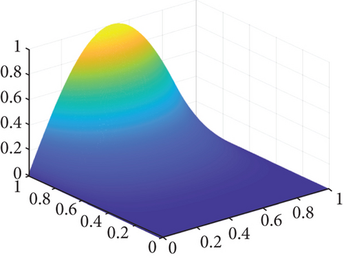
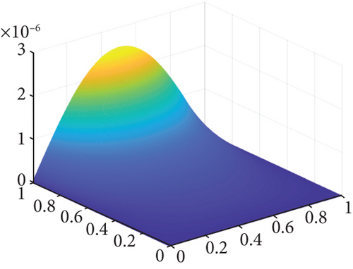
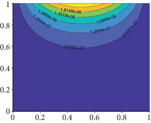
Figure 1 shows the exact solution, numerical solution, absolute error, and contour plot of absolute error with β = 0.5 at N = 1000 and M = 500. It demonstrates that the numerical solution of Equation (10) is in excellent agreement with the exact solution.

Example 10. In the second example, we consider the problem (2) with L = 1, T = 4 and u(0, t) = u(1, t) = 0, the source term as follows:

(40)

Details are in the caption following the image — **Figure 1 (a) Exact solution**
Open in figure viewer PowerPoint

Exact solution, numerical solution, absolute error, and contour plot absolute error for Example 9 with β = 0.5, M = 500, and N = 1000.

Then the corresponding initial term is u(x, 0) = sin(πx), and the exact solution is u(x, t) = sin(πx) − t⁴sin(2πx).

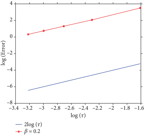
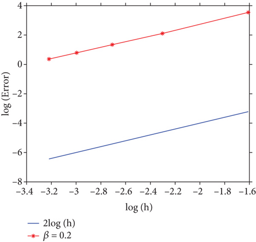
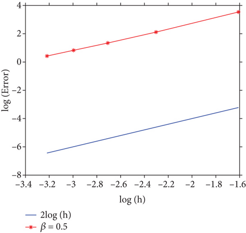
In Figures 2(a) and 2(b), we show the errors in L^∞-norm attain second order of accuracy in temporal direction for β = 0.2 and β = 0.5, respectively. In Figures 2(c) and 2(d), we show the errors in L^∞-norm attain second order of accuracy in spatial direction for β = 0.2 and β = 0.5, respectively. It is observed that the convergence order in the temporal and spatial directions are O(τ²) and O(h²), respectively, which are almost as the theoretical results in Theorem 7.

6. Conclusion

In this paper, we present two-level mesh method based on finite difference scheme to solve partial integro-differential equation. For the first step on coarse grid, we use finite difference method in time and global radial basis function finite difference in space. For the second step on fine grid, the finite difference method is used to solve the proposed problem, and the numerical solutions obtained by first step will be used as the initial conditions. The stability and error are discussed, and the convergence rate is obtained. Numerical examples show the efficiency of proposed scheme. It shows that the numerical results are in good agreement with theoretical analysis.

In our future work, we will study the numerical scheme of fractional derivatives, such as Riemann-Liouville derivative, Caputo derivative, and Caputo-Fabrizio derivative. Meanwhile, we would like to investigate fractional derivative in both time and space. In addition, we are interested to combine other numerical methods and RBF to consider the numerical solutions of high dimensional fractional integro-differential equations, irregular region problems, and nonlinear problems.

Conflicts of Interest

The authors declare that they have no conflicts of interest.

Acknowledgments

We are very grateful to both referees for carefully reading the paper and the most valuable comments and suggestions. This work is supported by the National Natural Science Foundation of China (No. 11861068), the Science Foundation for Distinguished Young Scholars of Xinjiang, China (No. 2022D01E13), and the Scientific Research Foundation for Outstanding Young Teachers of Xinjiang Normal University, China (No. XJNU202012).

Open Research

Data Availability

Data sharing not applicable to this article as no datasets were generated or analysed during the current study.

References

1 Volterra V., Theory of Functionals and of Integral and Integro-Differential Equations, 1959, Dover, New York, NY, USA.
Google Scholar
2 Patel V. K., Singh S., Singh V. K., and Tohidi E., Two dimensional wavelets collocation scheme for linear and nonlinear Volterra weakly singular partial integro-differential equations, International Journal of Applied and Computational Mathematics. (2018) 4, no. 5, 1–27, https://doi.org/10.1007/s40819-018-0560-4, 2-s2.0-85062713967.
10.1007/s40819-018-0560-4
Google Scholar
3 Singh S., Patel V. K., Singh V. K., and Tohidi E., Numerical solution of nonlinear weakly singular partial integro-differential equation via operational matrices, Applied Mathematics and Computation. (2017) 298, 310–321, https://doi.org/10.1016/j.amc.2016.11.012, 2-s2.0-85000785628.
10.1016/j.amc.2016.11.012
Web of Science® Google Scholar
4 Gurtin M. E. and Pipkin A. G., A general theory of heat conduction with finite wave speeds, Archive for Rational Mechanics and Analysis. (1968) 31, no. 2, 113–126, https://doi.org/10.1007/BF00281373, 2-s2.0-34250511985.
10.1007/BF00281373
Web of Science® Google Scholar
5 Miller R. K., An integrodifferential equation for rigid heat conductors with memory, Journal of Mathematical Analysis and Applications. (1978) 66, no. 2, 313–332, https://doi.org/10.1016/0022-247X(78)90234-2, 2-s2.0-0018031320.
10.1016/0022-247X(78)90234-2
Web of Science® Google Scholar
6 Nikan O., Avazzadeh Z., and Tenreiro Machado J. A., Numerical approach for modeling fractional heat conduction in porous medium with the generalized Cattaneo model, Applied Mathematical Modelling. (2021) 100, 107–124, https://doi.org/10.1016/j.apm.2021.07.025.
10.1016/j.apm.2021.07.025
Web of Science® Google Scholar
7 Nunziato J. W., On heat conduction in materials with memory, Quarterly of Applied Mathematics. (1971) 29, no. 2, 187–204, https://doi.org/10.1090/qam/295683.
10.1090/qam/295683
Web of Science® Google Scholar
8 Christensen R. M. and Freund L. B., Theory of viscoelasticity, Journal of Applied Mechanics. (1971) 38, no. 3, https://doi.org/10.1115/1.3408900.
10.1115/1.3408900
Google Scholar
9 Nikan O. and Avazzadeh Z., Numerical simulation of fractional evolution model arising in viscoelastic mechanics, Applied Numerical Mathematics. (2021) 169, 303–320, https://doi.org/10.1016/j.apnum.2021.07.008.
10.1016/j.apnum.2021.07.008
Web of Science® Google Scholar
10 Renardy M., Mathematical analysis of viscoelastic flows, Annual Review of Fluid Mechanics. (1989) 21, no. 1, 21–34, https://doi.org/10.1146/annurev.fl.21.010189.000321.
10.1146/annurev.fl.21.010189.000321
Web of Science® Google Scholar
11 Kim C. and Choi U., Spectral collocation methods for a partial integro-differential equation with a weakly singular kernel, The Journal of the Australian Mathematical Society. Series B. Applied Mathematics. (1998) 39, no. 3, 408–430, https://doi.org/10.1017/S0334270000009474.
10.1017/S0334270000009474
Google Scholar
12 Yan Y. and Fairweather G., Orthogonal spline collocation methods for some partial Integrodifferential equations, SIAM Journal on Numerical Analysis. (1992) 29, no. 3, 755–768, https://doi.org/10.1137/0729047, 2-s2.0-0026880680.
10.1137/0729047
Web of Science® Google Scholar
13 Qiao L. and Xu D., Compact alternating direction implicit scheme for integro-differential equations of parabolic type, Journal of Scientific Computing. (2018) 76, no. 1, 565–582, https://doi.org/10.1007/s10915-017-0630-5, 2-s2.0-85040689436.
10.1007/s10915-017-0630-5
Web of Science® Google Scholar
14 Tang T., A finite difference scheme for partial integro-differential equations with a weakly singular kernel, Applied Numerical Mathematics. (1993) 11, no. 4, 309–319, https://doi.org/10.1016/0168-9274(93)90012-G, 2-s2.0-0012661804.
10.1016/0168-9274(93)90012-G
Web of Science® Google Scholar
15 Luo M., Xu D., and Li L., A compact difference scheme for a partial integro-differential equation with a weakly singular kernel, Applied Mathematical Modelling. (2015) 39, no. 2, 947–954, https://doi.org/10.1016/j.apm.2014.07.014, 2-s2.0-84922663359.
10.1016/j.apm.2014.07.014
Web of Science® Google Scholar
16 López-marcos J. C., A difference scheme for a nonlinear partial integrodifferential equation, SIAM Journal on Numerical Analysis. (1990) 27, no. 1, 20–31, https://doi.org/10.1137/0727002, 2-s2.0-0025383598.
10.1137/0727002
Web of Science® Google Scholar
17 Sanz-Serna J. M., A numerical method for a partial integro-differential equation, SIAM Journal on Numerical Analysis. (1988) 25, no. 2, 319–327, https://doi.org/10.1137/0725022.
10.1137/0725022
Web of Science® Google Scholar
18 Sloan I. H. and Thomée V., Time discretization of an integro-differential equation of parabolic type, SIAM Journal on Numerical Analysis. (1986) 23, no. 5, 1052–1061, https://doi.org/10.1137/0723073.
10.1137/0723073
Web of Science® Google Scholar
19 Chen H., Gan S., Xu D., and Liu Q., A second-order BDF compact difference scheme for fractional-order Volterra equation, International Journal of Computer Mathematics. (2016) 93, no. 7, 1140–1154, https://doi.org/10.1080/00207160.2015.1021695, 2-s2.0-84925070773.
10.1080/00207160.2015.1021695
Web of Science® Google Scholar
20 Chen H., Xu D., Cao J., and Zhou J., A backward Euler alternating direction implicit difference scheme for the three-dimensional fractional evolution equation, Numerical Methods for Partial Differential Equations. (2018) 34, no. 3, 938–958, https://doi.org/10.1002/num.22239, 2-s2.0-85038247931.
10.1002/num.22239
Web of Science® Google Scholar
21 Chen H., Xu D., and Peng Y., A second order BDF alternating direction implicit difference scheme for the two-dimensional fractional evolution equation, Applied Mathematical Modelling. (2017) 41, 54–67, https://doi.org/10.1016/j.apm.2016.05.047, 2-s2.0-85003766132.
10.1016/j.apm.2016.05.047
CAS PubMed Web of Science® Google Scholar
22 Mohebbi A., Compact finite difference scheme for the solution of a time fractional partial integro-differential equation with a weakly singular kernel, Mathematical Methods in the Applied Sciences. (2017) 40, no. 18, 7627–7639, https://doi.org/10.1002/mma.4549, 2-s2.0-85062229504.
10.1002/mma.4549
Web of Science® Google Scholar
23 Qiao L., Xu D., and Wang Z., An ADI difference scheme based on fractional trapezoidal rule for fractional integro-differential equation with a weakly singular kernel, Applied Mathematics and Computation. (2019) 354, 103–114, https://doi.org/10.1016/j.amc.2019.02.022, 2-s2.0-85062155756.
10.1016/j.amc.2019.02.022
Web of Science® Google Scholar
24 Oruç Ö., A local radial basis function-finite difference (RBF-FD) method for solving 1D and 2D coupled Schrodinger-Boussinesq (SBq) equations, Engineering Analysis with Boundary Elements. (2021) 129, 55–66, https://doi.org/10.1016/j.enganabound.2021.04.019.
10.1016/j.enganabound.2021.04.019
Web of Science® Google Scholar
25 Oruç Ö., A strong-form local meshless approach based on radial basis function-finite difference (RBF-FD) method for solving multi-dimensional coupled damped Schrodinger system appearing in Bose-Einstein condensates, Communications in Nonlinear Science and Numerical Simulation. (2022) 104, article 106042, https://doi.org/10.1016/j.cnsns.2021.106042.
10.1016/j.cnsns.2021.106042
Web of Science® Google Scholar
26 Oruç Ö., A local hybrid kernel meshless method for numerical solutions of two- dimensional fractional cable equation in neuronal dynamics, Numerical Methods for Partial Differential Equations. (2020) 36, no. 6, 1699–1717, https://doi.org/10.1002/num.22499.
10.1002/num.22499
Web of Science® Google Scholar
27 Oruç Ö., Two meshless methods based on local radial basis function and barycentric rational interpolation for solving 2D viscoelastic wave equation, Computers & Mathematics with Applications. (2020) 79, no. 12, 3272–3288, https://doi.org/10.1016/j.camwa.2020.01.025.
10.1016/j.camwa.2020.01.025
Web of Science® Google Scholar
28 Oruç Ö., A radial basis function finite difference (RBF-FD) method for numerical simulation of interaction of high and low frequency waves: Zakharov-Rubenchik equations, Applied Mathematics and Computation. (2021) 394, article 125787, https://doi.org/10.1016/j.amc.2020.125787.
10.1016/j.amc.2020.125787
Web of Science® Google Scholar
29 Nikan O. and Avazzadeh Z., An improved localized radial basis-pseudospectral method for solving fractional reaction-subdiffusion problem, Results in Physics. (2021) 23, article 104048, https://doi.org/10.1016/j.rinp.2021.104048.
10.1016/j.rinp.2021.104048
Web of Science® Google Scholar
30 Li N., Tan Z., and Feng X., Novel two-level discretization method for high dimensional semilinear elliptic problems base on RBF-FD scheme, Numerical Heat Transfer, Part B: Fundamentals. (2017) 72, no. 5, 349–360, https://doi.org/10.1080/10407790.2017.1409511, 2-s2.0-85042484777.
10.1080/10407790.2017.1409511
Web of Science® Google Scholar
31 Xu J., A novel two-grid method for semilinear elliptic equations, SIAM Journal on Scientific Computing. (1994) 15, no. 1, 231–237, https://doi.org/10.1137/0915016.
10.1137/0915016
Web of Science® Google Scholar
32 Diethelm K., Ford N. J., and Freed A. D., Detailed error analysis for a fractional Adams method, Numerical Algorithms. (2004) 36, no. 1, 31–52, https://doi.org/10.1023/B:NUMA.0000027736.85078.be, 2-s2.0-4043121080.
10.1023/B:NUMA.0000027736.85078.be
Web of Science® Google Scholar
33 Guo J., Xu D., and Qiu W., A finite difference scheme for the nonlinear time-fractional partial integro-differential equation, Mathematical Methods in the Applied Sciences. (2020) 43, 3392–3412.
10.1002/mma.6128
Web of Science® Google Scholar
34 Abbasbandy S., Ghehsareh H. R., and Hashim I., Numerical analysis of a mathematical model for capillary formation in tumor angiogenesis using a meshfree method based on the radial basis function, Engineering Analysis with Boundary Elements. (2012) 36, no. 12, 1811–1818, https://doi.org/10.1016/j.enganabound.2012.06.011, 2-s2.0-84864364576.
10.1016/j.enganabound.2012.06.011
Web of Science® Google Scholar
35 Ghassabzadeh F. A., Tohidi E., Singh H., and Shateyi S., RBF collocation approach to calculate numerically the solution of the nonlinear system of qFDEs, Journal of King Saud University - Science. (2021) 33, no. 2, article 101288, https://doi.org/10.1016/j.jksus.2020.101288.
10.1016/j.jksus.2020.101288
Web of Science® Google Scholar
36 Schaback R., Error estimates and condition numbers for radial basis function interpolation, Adv. Comput. Math.(1995) 3, no. 3, 251–264, https://doi.org/10.1007/BF02432002, 2-s2.0-51249166702.
10.1007/BF02432002
Google Scholar
37 Yang Y., Soleymani F., Barfeie M., and Tohidi E., A radial basis function -- Hermite finite difference approach to tackle cash- or-nothing and asset-or-nothing options, Journal of Computational and Applied Mathematics. (2020) 368, article 112523, https://doi.org/10.1016/j.cam.2019.112523.
10.1016/j.cam.2019.112523
Web of Science® Google Scholar

All articles

Analysis of Two-Level Mesh Method for Partial Integro-Differential Equation

Abstract

1. Introduction

2. Construction of Numerical Scheme

3. Stability and Convergence

4. Two-Level Mesh Method for Integro-Differential Equation

5. Numerical Results

6. Conclusion

Conflicts of Interest

Acknowledgments

Open Research

Data Availability

References

Figures

References

Information

About Wiley Online Library

Help & Support

Opportunities

Connect with Wiley

Analysis of Two-Level Mesh Method for Partial Integro-Differential Equation

Abstract

1. Introduction

2. Construction of Numerical Scheme

3. Stability and Convergence

4. Two-Level Mesh Method for Integro-Differential Equation

5. Numerical Results

6. Conclusion

Conflicts of Interest

Acknowledgments

Open Research

Data Availability

References

Figures

References

Related

Information