[Retracted] Embedded Estimation Sequential Bayes Parameter Inference for the Ricker Dynamical System
Abstract
The dynamical systems are comprised of two components that change over time: the state space and the observation models. This study examines parameter inference in dynamical systems from the perspective of Bayesian inference. Inference on unknown parameters in nonlinear and non-Gaussian dynamical systems is challenging because the posterior densities corresponding to the unknown parameters do not have traceable formulations. Such a system is represented by the Ricker model, which is a traditional discrete population model in ecology and epidemiology that is used in many fields. This study, which deals with parameter inference, also known as parameter learning, is the central objective of this study. A sequential embedded estimation technique is proposed to estimate the posterior density and obtain parameter inference. The resulting algorithm is called the Augmented Sequential Markov Chain Monte Carlo (ASMCMC) procedure. Experiments are performed via simulation to illustrate the performance of the ASMCMC algorithm for observations from the Ricker dynamical system.
1. Introduction
Physical, biological, neuroscience, and object tracking systems are all examples of multidisciplinary fields in which the inference problems that govern the characteristics of nonlinear dynamical systems are applied [1–10]. The most commonly used statistical frameworks for finding solutions to parameter inference problems seem to be frequentist (or non-Bayesian) approaches that use maximum likelihood estimation (ML), such as the Expectation Maximization (EM) procedure [11–16]. It is computationally difficult to infer parameters for nonlinear dynamical systems using frequentist approaches. Furthermore, these procedures return just point estimates rather than the whole distribution, indicating parameter uncertainty. It is necessary to run the estimation method a large number of times, using uncertainty estimation techniques such as bootstrapping, to get estimates of uncertainty. This entails an increase in both the computational load and the intensity.
The posterior distribution of unknown parameters, on the other hand, is used to offer both a point estimate and a corresponding estimate of uncertainty when estimating unknown parameters using Bayesian approaches. The aim of Bayesian procedures in a dynamical system setup is to obtain the posterior of Ω, p(Ω|y1:T), given all observations up to the final time T, y1:Y. The posterior p(Ω|y1:T) is generally difficult to obtain in closed form, so Bayesian computational algorithms are utilized to approximate it in the Monte Carlo sense. Markov chain Monte Carlo (MCMC) methods are the most frequently used approaches for estimating the posterior distribution when closed forms are not accessible, and they are the most accurate. Although Bayesian computational methods may be used to derive the posterior distribution of an unknown parameter, they are only justified in the limiting sense and can require a significant number of burn-ins before the MCMC algorithm converges [17–19]. In spite of this, certain computational methods are trivial to conceive and execute on computers, and standard packages are already available for many uncomplicated implementations of these procedures [20–22]. Some of the MCMC procedures are the Metropolis-Hastings (MH) algorithm, Gibbs sampler, and particle Markov Chain Monte Carlo (PMCMC) [23–25].
Several sequential Monte Carlo (SMC) approaches have been developed to address the constraints of the Markov Chain Monte Carlo (MCMC) algorithm for parameter estimation in dynamical systems. It is the core concept of SMC to utilise important samples to estimate the posterior of Ω at each k point in time and to propagate the samples sequentially via a suitable kernel. There exists an extensive literature on SMC methods (see, for example, [26–29]). The SMC-based parameter inference in nonlinear dynamical systems was first addressed in [30] where the Liu and West filter was developed. An artificial evolution of parameters for parameter Ω is used in the Liu and West filter and assumes a mixture of normal distribution for the posterior distributions, p(Ω|y1:k), for k = 1, 2, ⋯, T within the mixture distribution. The tuning parameters govern the extent of the control of overdispersion of the mixture components [30, 31]. To minimize the weight degeneracy or particle decay, the main idea is to generate new samples from the posterior by fitting the mixture to the posterior. The Liu and West filter can generally be applied to any dynamical system, which is the main attraction of this procedure. However, due to the artificial evolution of the unknown parameter, the artificial variability is incorporated, which is the main drawback of this algorithm.
The aim of Bayesian procedures is to obtain the posterior of Ω, p(Ω|y1:T), given all observations up to time T, y1:T. The posterior p(Ω|y1:T) is again difficult to obtain in close form, so Bayesian computational algorithms are utilized to approximate it in a Monte Carlo sense.
Another major class of SMC methods for parameter inference that does not introduce overdispersion in the posterior of Ω is particle learning algorithms [32, 33]. The original method is attributed to Storvik [34, 35] resulting in Storvik’s filter (similar approaches are also proposed in [36, 37]). Storvik’s filter assumes that the posterior distribution of Ω given m0:k and y0:k depends on a lower-dimensional set of sufficient statistics that can be recursively updated for each k = 1, 2, ⋯, T. This recursion for sufficient statistics is defined by sk+1 = S(sk, mk+1, yk+1), leading to the generation of Ω samples according to Ω ~ p(Ω|m0:k, y1:k) = p(Ω|sk) for each k = 1, 2, ⋯, T. Unlike the Liu and West filter, in Storvik’s filter, there is no artificial evolution process for Ω and thus it does not suffer from overdispersion [38]. However, the crucial assumption in Storvik’s filter is the availability of sufficient statistics sk as well as the ability of sampling from the posterior p(Ω|sk) given the sufficient statistics sk.
Subsequent developments in SMC methods for parameter inference have extended the applicability of Storvik’s filter to a variety of more general settings (see, for example, [39, 40]). The extended Liu and West (ELW) filter to estimate parameters and states [40] divides the parameter set to be inferred Ω, into two sets, Ω0 and γ representing parameters without and with sufficient statistics, respectively. For the Ω0 set, the ELW filter uses the Liu and West filter, where an artificial random error is introduced to the static parameter Ω0. The set of parameters γ updated based on Storvik’s filter γ ~ p(γ|sk(Ω0). The sufficient statistics sk(Ω0) are based on the static parameters. The rest of the parameters have the artificial evolution in which overdispersion is used. The overall set of parameters is represented as Ω = (Ω0, γ). The ELW filter applies to a wider class of state space models compared to Storvik’s original procedure but suffers from two drawbacks, namely, (i) artificial overdispersion of the final posterior and (ii) the requirement of the existence of the sufficient statistic sk(Ω0) for γ and the ability of sampling from the posterior p(γ|sk(Ω0)).
Development of statistical methods in specific ecological combines the nonlinear and near chaotic behavior of the system response for various applications [41–44]. A detailed comparison of the inference problem for nonlinear ecology and epidemiology is given in [45]. Nonlinearity is an observer in the experimental research [46]. Although the objectives of epidemiologists and ecologists are different, both are concerned about the persistence of specific species. The mathematical explanations of the population dynamics are similar in both studies [45].
The aim and scope of this paper are to use the chaotic epidemiological or ecological model and perform parameter inference. There are two objectives. First is to perform the inference for the proposed application even if sufficient statistics are not available. Second is to use an online method to perform the parameter inference. Many researchers [47, 48] have discussed the relationship between statistics and chaos. The primary inference methodology used in this manuscript is developed in [49], which is a sequential MCMC (SMCMC) procedure to obtain the unknown parameter posterior inference in dynamical systems. However, then in [49], the proposed methodology was only applicable when the considered measurement model is linear and additive Gaussian noise. In this work, the measurement model of the Ricker dynamical system incorporates a non-Gaussian distribution, and the associated dynamical system (a special case of (1) and (2)) incorporates nonlinearities via the transfer function Φk−1,Ω(·). The appropriate SMCMC algorithm for inferring Ω is developed for the Ricker dynamical system subsequently.
The remainder of this paper is organized into the following sections: In Section 2, Ricker’s model is discussed. In Section 3, details of the SMCMC procedure are given. The simulation experiments are given in Section 4. In the last section, Section 5, we state our conclusions, and potential future work is discussed.
2. Ricker’s Model
Theoretical ecology relies heavily on mathematical models of competition. Several mathematical models have been suggested to date to characterize the growth of contending populations; some of them are detailed in [50–52], including discrete-time models [53, 54]. The wide range of biological factors that influence ecosystem behavior makes it difficult for researchers to come to a consensus on how to simulate the dynamics of competing populations. Numerous instances of competing species and techniques for mathematical modelling are discussed in one of the pioneering publications on interspecific interaction [55]. The scramble competition has been found to fit the Ricker model [56, 57]. From order to chaos, the Ricker model illustrates dynamics [20–58]. It would be fascinating to observe what dynamic modes emerge when two Ricker maps are joined.
Here yk is the measurement parameter of the individual sampled at any time point k, and ϕ is the scale parameter.
Using the transformed variables, equations (5) and (6) can be seen to be special forms of the general state space and measurement model equations given by (1) and (2), respectively. We have Φk−1,Ω(·) = log(r) + log(mk−1) − mk−1, and Ψk,Ω(·) is the Poisson probability density function with mean . Thus, the Ricker dynamical system has three underlying parameters that govern the system, namely, σ2, log(r), and ϕ. In this paper, the latter two parameters are taken to be unknown, that is, Ω = [log(r), ϕ] and σ2 = 0.09 is assumed fixed and known. True values of the parameters for our simulation studies are taken to be Ω = [log(r), ϕ] = [3.8,0.7], which the same as given in [45].
3. An Augmented Sequential Markov Chain Monte Carlo Algorithm
Sequential Markov chain Monte Carlo algorithm working process is described in the subsequent text. Sequential updating characteristic of SMCMC is used in the proposed technique. The core notion is addressed in [59], which is focused on the Monte Carlo sum, but the cumulative filtering steps required for estimating the probability p(yk|y1:k−1, Ω) minimise. State variable mk and unknown parameter Ω are supplemented at the time step of k − 1 in [49]. Therefore, the likelihood function changes accordingly from p(yk|y1:k−1, Ω) to p(yk|mk−1, Ω). It is possible to achieve the analytical expression to avoid the need for cumulative filtering procedures. This is particularly useful when the amount of k is substantial.
The ASMCMC is an iterative procedure that starts from the initial time step k = 1, increases sequentially, and finally ends when k = T. Within the k-th step of the ASMCMC procedure, posterior samples are obtained based on an underlying Markov chain Monte Carlo procedure. This Markov chain Monte Carlo procedure will be called the k-th time step Markov chain Monte Carlo procedure. The target of the k-th step MCMC procedure is the posterior, p(Ω, mT|y1:k), at time step k. Thus, when k = T, we will have obtained samples from the desired posterior p(Ω, mT|y1:k) as well as p(Ω, |y1:k) via marginalization. Details on the implementation of the k-th step Markov chain Monte Carlo procedure are as follows.
To initialize the k-th time step MCMC procedure, the M samples are taken to form the starting points of Mk-th step MCMC procedures, that is, and for j = 1, 2, ⋯, M. Some notations are developed here: denoted by and , respectively, to be the values of Ω and mk−1 at the g-th cycle of the k-th time step MCMC procedure initialized by for j = 1, 2, ⋯, M. In other words, the Mk-th time step MCMC procedures initialized based on form separate chains based on separate starting values; this entails that the M MCMC chains can be run in parallel for each time step k = 1, 2, ⋯, T.
- (i)
Generate
- (ii)
Compute the acceptance probability
Continue the iteration from k + 1⟶k + 2.
-
Algorithm 1: Augmented sequential MCMC procedure.
-
=ASMCMC
-
Initialize with M initial value prior density
-
p0(Ω, m0).
-
Start for k=1:T
-
=AMCMC
-
DO: M Parallel MCMC chains initialized from M pairs , j = 1, 2, ⋯, M.
-
For the generic j-th chain:
-
Start with (prior value).
-
for k=1:B (burn-in chains)
-
Generate samples (Ω∗, m∗)~
-
q(Ω∗, m∗|Ωk−1, mk−1).
-
Compute the acceptance probability
-
αk = min{A · B, 1} as in (9) and (10).
-
Set (Ωg, mg) = (Ω∗, m∗) with
-
probability αk
-
Else (Ωg, mg) = (Ωk−1, m(k − 1))
-
with probability 1 − αk
-
end for
-
Obtain , from j = 1, 2, ⋯, M
-
chains.
-
Samples are based
-
(12)
-
Mixture fitting
-
Output: and fitted mixture model .
-
The posterior distribution p(Ω|y1:T) is based on the collected samples of .
-
end for
4. Results and Discussion
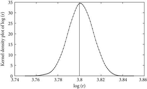
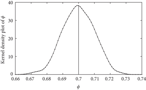
In this section, the ASMCMC methodology is used for parameter inference in the Ricker dynamical system. The y-observations were generated from the time-discretized Ricker’s model (state space model given by (5) and the measurement model given by (6)) using the initial point mass prior at m0 = 7. Starting from the initial state values generated from the prior, the state and measurement systems are updated at every fixed time step of k = 1, 2, ⋯, T = 10. The true value for Ω is taken as Ω = [log(r), ϕ] = [3.8,0.7], which is the same as the choice made in [45]. The burn-in B was set at B = 5000. The estimated posterior density curves are obtained based on the final posterior samples of Ω = [log(r), ϕ] at the completion of the ASMCMC algorithm. These density curves are given in Figures 1 and 2 for the parameters log(r) and ϕ, respectively. In Figure 1, estimated density curves based on final posterior samples of the parameter log(r) at the completion of the ASMCMC are presented. The vertical solid black line represents the true value of the parameter log(r) = 3.8, whereas the estimated density curves based on the final posterior samples of the parameter ϕ at the completion of the ASMCMC are presented in Figure 3. The vertical solid black line represents the true value of the parameter ϕ = 0.7. We note that the true values of the parameters are well within the support of their respective posterior densities, which gives credence to the parameter inference methodology using the ASMCMC procedure. The following Table 1 represents the simulation parameters considered in the experimental setup.


| Variable | Value | Description |
|---|---|---|
| log(r) | 3.8 | True value of parameter |
| ϕ | 0.7 | True value of parameter |
| m0 | 7 | Prior of state variable |
| B | 5000 | Burn-in period |
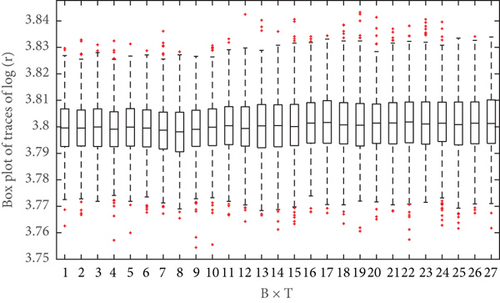
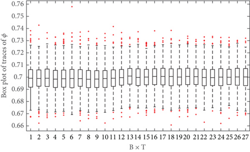
To illustrate the convergence of the ASMCMC procedure, boxplot trajectories represent the distribution of p(Ω|y1:k) for k = 1, 2, ⋯, T can be plotted. These boxplots are constructed based on the M final iteration for j = 1, 2, ⋯, M, collected after burn-in. Figure 3 shows that the boxplot trajectories based on posterior samples of log(r). Figure 3 indicates that these boxplot trajectories have stabilized long before reaching the final time point T = 10. In other words, the posterior p(log(r)|y1:k) changes much when k approaches the final time point T, which can be taken as an indication that the estimate of p(log(r)|y1:k) based on the ASMCMC sampler has converged. A similar boxplot trajectory plot (shown in Figure 4) is obtained for ϕ which indicates that the convergence of its posterior distribution has been achieved.

5. Conclusion
The dynamical system based on Ricker’s model is an example of a nonlinear and non-Gaussian system that has applications in ecology and epidemiology. We develop the ASMCMC algorithm for the Ricker dynamical system to perform Bayesian parameter inference. We observe that the posteriors encompass the true parameter values used to simulate observations from the Ricker dynamical system. Our future work will be to investigate the performance of the ASMCMC algorithm when σ2 is unknown as well and for high-dimensional dynamical systems that appear in ecology and epidemiology.
Symbols
-
- mk:
-
- State variable
-
- yk:
-
- Observation variable
-
- Φk−1,Ω(·):
-
- State model
-
- Ψk,Ω(·):
-
- Measurement model
-
- T:
-
- Final time point
-
- k:
-
- Time variable
-
- uk−1:
-
- State noise
-
- vk:
-
- Observation noise
-
- Ω:
-
- Unknown parameters
-
- p(·|·):
-
- Probability density function
-
- q(·|·):
-
- Proposal distribution
-
- y1:k:
-
- Observation vector for time point 1 to k
-
- sk:
-
- Sufficient statistics at k-th time point
-
- :
-
- Weights vector at time point k
-
- B:
-
- Burn-in period
-
- {log(r), ϕ}:
-
- Unknown parameters of Ricker dynamical system
-
- :
-
- Augmented particles of unknown state and parameters.
Conflicts of Interest
Authors of this article have no conflict of interest publishing this article in Journal of Sensors.
Open Research
Data Availability
This paper does not require any dataset whereas the simulated data is used using MATLAB tool.


