In this manuscript, a giving-up smoking model is develop using bilinear incidence rate, harmonic mean type of incidence rate and keeping in view the relapse factor associated to smoking. It is shown that the model' solution is bounded and positive for the appropriate initial data. The equilibria of the model are obtained, and it is proved that the smoking-free equilibrium is both locally and globally asymptotically stable for R₀ less than unity. It is shown that the model has a positive light smoker present equilibrium whenever R₀ is greater than one, and it is locally asymptotically stable if we have 1 < R₀ < 1 + 2β₁(μ + d + δ)/Λβ₂. Conditions for the global stability of light smoker present equilibrium are rigorously investigated. Also, it is proved that the model has a smoking present equilibrium when R₀ satisfies some condition which is investigated both for local and global behavior. By considering a few control measures, optimal control strategies are achieved with the help of Pontryagin’s maximum principle. The analytical results are verified numerically, and effectiveness of the control program is presented.

1. Introduction

Among other diseases, infectious diseases are the most alarming threat to humanity from the last few centuries. The plague of Athens is considered to be the first ever epidemic which affects human life to a great extent [1, 2]. The life in Egypt and Roman was completely demolished by the smallpox in 165-180 C.E. in which millions of people died [3]. The epidemic Black Death in Europe is observed to be the first well-documented epidemic which killed more than 50 millions of people that region and Mediterranean. Various other epidemics affected human life throughout the history, and the current corona virus disease is the last epidemic whose disasters are in front of us. Thus, it is very crucial to understand the dynamics of such infectious disease (particularly the emerging epidemics) and to control its spread in early transmission phase. In the context of these extensive illnesses, the tobacco pandemic is one of the world’s most serious health threats. According to statistics, up to 50% of smokers die as a result of their habit, a tobacco-related mortality occurs every 8 seconds, and 10 percent of the adult population dies as a result of tobacco-related illnesses [4].

Smoking habit grows and spreads across a society in the same way as an epidemic illness does, and generally, it nearly follows the same process. To be specific, people are prone to smoking at first, then become active users, and eventually recover through certain control methods or self-abandonment of its usage. In the early twentieth century, William Hamer’s work on mathematical modeling of infectious illnesses achieved substantial progress. Perhaps, Hamer was the first who introduces mass action law in epidemic modeling. However, Sir Ronald Ross is considered the father of today’s mathematical biology due to his work on malaria. In 1911, he published a book regarding malaria in which he used mathematical models for describing the dynamics of the infection and calculated the threshold parameters. The formal mathematical biology started with the work of Kermack and McKendrick [5], and then, significant contributions were made in the subject, for instance, one can see [6–11].

To study the transmission of smoking habits and its control in the society, numerous researchers used the tools of mathematical modeling and optimal control theory. Castillo-Garrsow et al. [12] used a model of SIR type and well-presented the qualitative aspects of the model under discussion. Sharomi and Gumel [13] extended the work of Castillo-Garrsow et al. and introduced temporary quit class into the model. Zaman [14] incorporated the light smoker compartment and rigorously investigated the model from mathematical perspectives. Subsequently, considering various features and characteristics of smoking, sophisticated models have been developed and investigated, for example, [15–18].

Incidence rate plays a crucial role while investigating the dynamics of any epidemic disease. The bilinear and saturated incidence rates were widely used in case of epidemic diseases and smoking models, for instance, one can see [12, 19, 20]. The authors in [17, 21, 22] used the square root incidence rate and discussed the models from various mathematical aspects. In the sequel, Rahman et al. [4] used harmonic mean type of incidence rate in his giving-up smoking model, investigated the dynamics of the model, and set the controlling strategies for reducing the smoking habit. Similarly, Alzaid and Alkahtani used the same incidence rate and studied the effect of relapse [23]. This work as well as the work of Rahman et al. assumed that potential smokers will start smoking only if they make a contact with light smoker. However, this is usually not the case. A person (potential smoker) may start smoking when he/she comes into contact with a smoker. In this work, the authors intend to overcome this gap. We shall assume that smoking habit may spread in the population via two roots; (i) contacts of potential smoker and light smokers and (ii) contact between smoker and light smokers. For the former type of spread, we will use the usual harmonic mean type of incidence rate, and for the later, the standard bilinear incidence rate will be utilized. By doing so, the present model will cover models [4, 23] as a subcase.

The rest of the work is organized as follows. The model formulation and essential biological features to the model are discussed in Section 2. The smoking generation number and equilibria of the model are presented in Section 3. We investigated the local stability of each equilibrium point in Section 4, whereas the criteria for global dynamics of smoking-free, light smoker present, and smoking-present equilibria are derived in Section 5. The local sensitivity will be performed in Section 6. Based on sensitivity analysis, we take into account some control variables and formulated a control problem for further analysis in Section 7. The desired goals were obtained, and the results are verified through simulations in Section 8. Finally, we presented the conclusion of the work.

2. Model Formulation and Well-Posedness

To formulate the model, we will divide the entire population into four compartments, namely, the potential smokers P = P(t), the light (or occasional) smokers L = L(t), the smokers S = S(t), and the quit smokers Q = Q(t). That is, if T(t) denotes the total population, and then, T(t) = P + L + S + Q. We assumed that smoking habit spread in the population through (i) contact between potential smokers and light smokers and (ii) contact between the light smokers and chain smokers. The former contact is mathematically described by harmonic mean type of incidence rate. The reason for taking such type of contact is that the potential smokers may start smoking at a slower rate whenever they come into contact with the light smokers. Due to tendency of light smokers towards smoking, the light smokers will come into contact with smokers frequently and the rate will obey the mass action law. Hence, we assumed the bilinear incidence rate between light smokers and smokers. Furthermore, the harmonic mean type of incidence rate takes into account the behavioral changes of potential smokers and the crowding effect of the light smokers which prevent the unboundedness of the contact rate by choosing suitable parameters. Also, it is very hard to become a light smoker (because many social/cultural variables can restrict the contacts of light smokers with potential smokers), and mathematically, this phenomenon can be modeled by using the harmonic mean type of incidence rate instead of using bilinear incidence rate (because PL/P + L ≤ PL whenever P and L are positive). Besides this type of spread, we take into account the spread arising from contact between potential smokers and smokers which is described by bilinear incidence rate. It is also assumed that the quitting of smoking is not permanent, and an individual may start smoking again. These assumptions lead to the following system of ODEs representing the dynamics of smoking habit in a population.

(1)

with initial conditions

(2)

where P₀, L₀, S₀, and Q₀ stand for the initial size of the population of the respective compartments. The description of parameters used in model (1) is shown in Table 1.

Table 1. Interpretation of parameters of model (1).

Parameter	Interpretation
Λ	Constant recruitment into the potential smokers
β₁	The contact rate of occasional and potential smokers
β₂	The contact rate between smokers and light smokers
μ	The natural mortality rate
d₀	Death rate due to smoking
δ	Temporarily quitting rate of smokers

By adding the governing equations of model (1), we obtain the conservation law

(3)

with T(0) = T₀ = P₀ + L₀ + S₀ + Q₀.

Theorem 1. For the nonnegative initial data, if a solution to model (1) exists, it must be positive.

Proof. Consider the second equation in model (1), and its solution is given by

(4)

By using this relation in the third equation of system (1), we have S(t) ≥ 0 which assures the positivity of Q(t). Finally, using these facts in the first equation, we have P(t) ≥ 0.

Theorem 2. For nonnegative initial conditions that are not identically zero on any interval, all possible solutions of system (1) are bounded in the region

(5)

Since each compartment denotes the size of population and thus must be nonnegative, the desired solution space is

. Thus, the each component in the vector (P(t), L(t), S(t), Q(t)) is bounded below by zero, and thus, we have to find the upper bound for the solution. From the conservation equation (3), we have

(6)

By solving this differential inequality, we get

(7)

Letting t⟶∞, we get T(t) ≤ Λ/μ. Thus, all solutions of the model are bounded by 0 and Λ/μ, and hence, the desired feasible set is (4).

Theorem 3. For system (1), the nonnegative space is positive invariant.

Proof. Consider the vector Ψ = (P, L, S, Q); then, in matrix form, we can write model (1) in the form

(8)

where

(9)

Clearly, the nondiagonal entries of matrix are nonnegative which guarantees that is Metzler matrix [24]. Further, , and thus, system (1) is positively invariant in the desired space. In the next section, we intended to find the smoking generation number (an important parameter describing the behavior of a system) as well as the possible equilibria of the proposed system.

3. Equilibria of the Model and Smoker Generation Number

In order to find the equilibria of the proposed model (1), we set

(10)

(11)

(12)

(13)

System of equations (10)–(13) always has a solution of the form

(14)

This fixed point is known as smoking-free equilibrium of the model.

To calculate the smoker generation number, we will follow the procedure of [25]. For this purpose, consider the smoker classes from system (1) and assume y = (L(t), S(t))^T, that is,

(15)

where

(16)

Considering the Jacobians of these two matrices at DFE, we get

(17)

and thus,

(18)

Let us consider

; thus,

(19)

Since R₀ (the smoking generation) is the dominant eigenvalue of the next generation matrix

, hence

(20)

By using the number R₀, we can obtain other possible equilibria of system (1) using equation (3).

Theorem 4.

(1)
If R₀ > 1, then model (1) has a positive light smoker present equilibrium given by

(21)

(2)
If R₀ < 1, then the model has a smoking-free equilibrium given by (14)
(3)
Whenever R₀ = 1, then again, the model has the smoking-free equilibrium given by (14)

Proof. By solving systems (10)–(13) and keeping in view that there are no smokers (i.e., S(t) = 0) in the community, we obtained the light smoker present equilibrium (21). However, for R₀ < 1, the light smoker becomes negative and hence, the model will have just the smoking-free equilibrium (14). In the similar way, if we assume R₀ = 1, then the fixed point (21) becomes the smoking-free equilibrium as we have Λ/2β₁ = Λ/(μ + d)R₀.

Theorem 5. There exists a positive smoking present equilibrium of model (1) blue if R₀ ≥ 1 and β₂S_∗ < μ + d.

Proof. System (1) has a positive solution of the form

(22)

where

(23)

and S_∗ is a positive root of

(24)

which surely exist by Descartes’ rule of signs whenever R₀ > 1 and β₂S_∗ < μ + d. Further, if we set R₀ = 1, then both solutions of equation (24) are positive and real and hence the theorem.

4. Local Stability Analysis of Equilibria

To find out the local stability of system (1) at each equilibrium point, first, we will calculate the Jacobian matrix

(25)

Theorem 6. The SFE (14) of system (1) is locally asymptotically stable for R₀ < 1.

From relation (25), the Jacobian of system (1) at E₀ is given by

(26)

Matrix (26) has eigenvalues t₁ = −(μ + d), t₂ = −(μ + d + δ), t₃ = 2β₁ − (μ + d), and t₄ = −(μ + d + γ). As the parameters of the model assume positive values, thus the eigenvalues t₁, t₂, and t₄ are negative and t₃ = (μ + d)(2β₁/μ + d − 1) = (μ + d)(R₀ − 1) is negative only if R₀ < 1. Hence, for R₀ < 1, all of the eigenvalues of the Jacobian matrix at E₀ are negative and so E₀ is locally asymptotically stable. Further, if R₀ = 1, then t₃ = 0. However, if we assume R₀ > 1, then E₀ becomes unstable as one of the eigenvalues is positive in such case.

Theorem 7. The local smoking present equilibrium (LSPE) (21) of system (1) is locally asymptotically stable for 1 < R₀ < 1 + 2β₁(μ + d + δ)/Λβ₂.

Proof. From relation (25), the Jacobian of system (1) at E_l is given by

(27)

The eigenvalues of matrix (30) are t₁ = −(μ + d), t₂ = −(μ + d)(R₀ − 1), t₃ = −(μ + d + γ), and t₄ = (R₀ − 1)Λβ₂/2β₁ − (μ + d + δ). Now, for positive parameters of the model and for R₀ > 1, the eigenvalues t₁, t₂, and t₃ are negative. However, t₄ is negative only for R₀ < 1 + 2β₁(μ + d + δ)/Λβ₂. Hence, if 1 < R₀ < 1 + 2β₁(μ + d + δ)/Λβ₂, all of the eigenvalues of the Jacobian matrix at E_l are negative and so E_l is locally asymptotically stable. Moreover, for R₀ = 1, we have t₂ = 0. In the case of R₀ < 1, t₂ becomes positive and thus, the equilibrium E_l will be unstable.

Theorem 8. The smoking present equilibrium (SPE) is locally asymptotically stable of if 1 < R₀ < 1 + β₂S_∗/μ + d.

Proof. The Jacobian at SPE is given by

(28)

where

(29)

(30)

(31)

(32)

(33)

(34)

The characteristic equation of matrix (28) is given by

(35)

Clearly, a₁₁, a₁₂, a₂₁, a₃₂, and a₄₄ are positive and

(36)

only if β₂S_∗ > (d + μ)(R₀ − 1). Thus, all of the coefficients of the characteristic equation (35) are positive, and hence, by Descartes’ rule of signs, this equation has no positive real solution. By using −τ in place of τ in equation (35) and utilizing Descartes’ rule of signs, we get that all of the eigenvalues of this equation are negative or complex conjugates with dominant negative real part. Therefore, the SPE is locally asymptotically stable whenever R₀ < 1 + β₂S_∗/μ + d. Further, for the existence of SPE, we must assume that R₀ > 1. Moreover, the case R₀ = 1 does not affect the stability of the equilibrium point; however, this condition will challenge the existence of smoking-present equilibrium.

5. Global Stability Analysis of the Equilibria

Theorem 9. Let R₀ ≤ 1; then, the smoking-free equilibrium (SFE) E₀ of model (1) is globally asymptotically stable (GAS).

Proof. For proving the required result, the Lyapunov function of the following form is assumed:

(37)

By considering the derivative of (37) with respect to time t and using model (1), we have

(38)

because P(t)/P(t) + L(t) ≤ 1. Thus,

(39)

Hence,

(40)

only if R₀ ≤ 1, and thus, by LaSalle’s invariant principle [26], E₀ is globally asymptotically stable in the feasible region.

Theorem 10. If 1 < R₀ < β₂Λ + 2β₁(d + μ)/β₂Λ, then the local smoking present equilibrium (LSPE) E_l of model (1) is globally asymptotically stable (GAS).

Proof. To prove the main result, we will take into consideration the Lyapunov function of the form

(41)

By considering the derivative of (37) with respect to time t and using model (1), we have

(42)

for R₀ > 1 and so by LaSalle’s invariant principle, the light smoker present equilibrium E_l is globally asymptotically stable. By considering relation (42) and the case of R₀ = 1, we will reach to the conclusion of Theorem 9 (as the case of R₀ = 1 does not guarantee the existence of LSPE).

Theorem 11. If R₀ > 1, β₂S_∗ < μ + d and , then (1) is GAS at SPE E_∗.

Proof. By considering the Jacobean (25) of the system at the SPE, we have

(43)

The third additive compound matrix of J_∗ is given by

(44)

where

(45)

Consider ρ(χ) = diag{Q, S, L, P} such that ρ(χ⁻¹) = diag{1/Q, 1/S, 1/L, 1/P} and time derivative is Therefore,

(46)

and hence,

(47)

By defining B = ρ_fρ⁻¹+^∣2∣ρ⁻¹ so that

(48)

where

(49)

Consequently,

(50)

Now we have

(51)

By combining the preceding four inequalities, we have the following inequality.

(52)

and we denote the Lozinskii measure by μ(B) = h_i, i = 1, 2, 3, 4, and hence, it shows that the SPE is GAS.

6. Local Sensitivity Analysis

The term R₀ is generally influenced by the inconsistencies in data gathering and estimated values. Sensitivity analysis is used to assess the relative impact of epidemic factors for disease propagation and control.

Definition 12. For the basic reproduction number, the normalized sensitivity index of a parameter ψ (which depends on the partial derivative of R₀ w.r.t ψ) is of the following form:

(53)

By calculating the sensitivity index, we may determine R₀’s responsiveness. To find the sensitivity of each parameter for R₀, we will employ equation (53) which was suggested by Tilahun et al. [27]. On the basis of parameter values β₁ = 0.006, d = 0.00004, and μ = 0.08, we have the sensitivity indices of the form

(54)

These indices enable us to determine the relevance of numerous variables involved in disease transmission, as well as the relative change in the number of reproductions as a function of parameter changes. Using such indices, we may identify the characteristics that have a significant impact on R₀ and are critical for disease prevention.

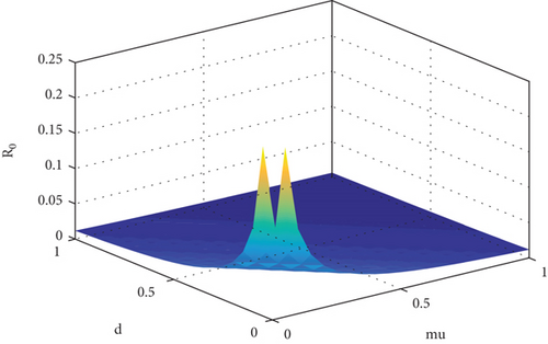
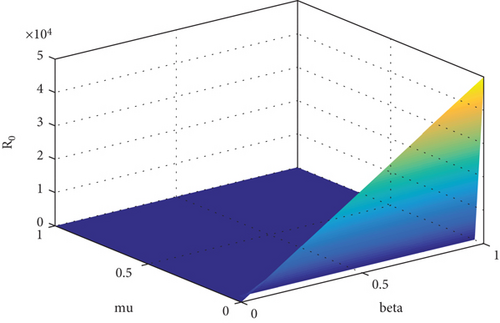
Table 2 suggests that there is a positive relation between R₀ and β₁ while negative influence of μ and d on R₀. The same argument is supported by Figure 1. This means that if you raise or reduce the value of parameter β₁ by 10%, it will rise or decrease R₀ by 10%. Similarly, if we reduce or increase μ and d by 1 percent, its relative inverse impact on R₀ will be 99.9% and 0.04%, respectively. To prevent smoking from the population, we must consider those parameters which have high sensitivity indices. Based on the sensitivity indices, we concluded that β₁ will directly affect R₀ (100%) whereas μ affects R₀ inversely about 99%. Thus, to reduce smoking habit, we must focus on the contacts between potential smokers and light smokers. It is simple to develop a control mechanism program for eradication of smoking habit based on this study.

Table 2. Sensitivity indices of R₀ w.r.t and the parameters β₁, μ, and d.

Parameters	Sensitivity index	Value
β₁		1
μ	S_μ	−0.999500
d	S_d	−0.00049975

Details are in the caption following the image — **Figure 1 (a) R0 verses μ and d at fixed β1 = 0.006**
Open in figure viewer PowerPoint

Sensitive parameters β, μ, and d and its impact on R₀.

7. Formulation and Analysis of Optimal Control Problem

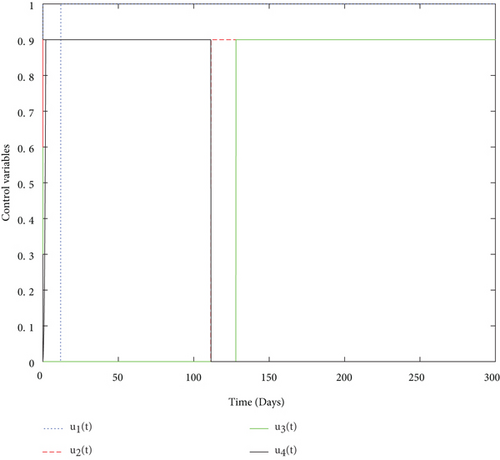
In this part, we simulate the eradication of smoking habit from the population by using the tools of control theory [9, 28]. We focus on reducing transmission, which has a sensitivity index of 1, to develop a control plan based on local sensitivity analysis. Further, to make the control program more effective, we take into consideration the following four control measures.

The first control measure is the education campaign which is denoted by u₁(t), and its aim is to reduce the size of potential smokers. The second control variable u₂(t) shows physically antismoking gum, and it will reduce the number of light smokers. The third and fourth control variables are antinicotive drug u₃(t) and ban on smoking particularly in public places by the government u₄(t). These measures will be imposed on the smoking compartment. It is observed that whenever the law enforcement personnel came into contact with light smokers (which smoke in public places), the light smokers will tend to quit smoking in public places. That is, by increasing the law enforcement personnel in public places, the size of light smokers will tend to decrease and hence, small number of individuals will tend to quit smoking. Therefore, we will use the term 1 − u₄(t) which will reduce the contacts between the law enforcement personnel with the light smokers. The control variables are subject to some conditions;

for i = 1, ⋯, 4 and u₁ ≤ u₄ ≤ u₂ ≤ u₃. These control variables are the main measures which could help in reducing the smoking habit [29]. Based on the control measures, we have the following governing equations for the control problem:

(55)

with the conditions

(56)

Our optimum control strategy is to reduce/minimize the number of potential smokers, light smokers, and smokers while increasing the number of people who quit smoking. Keeping in view the control problem (55), our cost functional is given by the following:

(57)

In the cost functional (57), D_i’s are positive constants describing the balancing factors, whereas F_i’s are the cost associated to the control measures. Clearly, the cost functional has a goal to reduce smoker population and to enhance the size of quit smokers. Our main focus is to find a set of functions

in such a way that

(58)

where the set V is the admissible control set and is define by

(59)

where u_i(t) are the control variables described above, and these are Lebesgue measurable functions. To identify such control measures, we must first establish that actually they exist.

7.1. Existence of Solution to the Control Problem

For proving the desired result, we will take into consideration problems (55) and (56) and will show that actually this system has a solution. It is worthy to notice that nonnegative bounded solutions to the state system exist if we have bounded Lebesgue measurable control measures and nonnegative initial conditions [28]. Let

(60)

and here,

(61)

Equation (60) denotes a nonlinear system (the proposed control problem) with bounded coefficients. Set

(62)

By considering the following,

(63)

where N₁ = max(2β₁, β₂) is free from the state’s variable. Also, one can write

(64)

where

; thus,

is uniformly continuous function in the sense of Lipschitz. Further, for the definition of the control measures and conditions on the states (P(t) > 0, L(t) ≥ 0, S(t) ≥ 0 and R(t) > 0), we can observe that a solution to the control problem (55) does really exist. The following conclusion holds for the existence of control variables in the optimum control problem.

Theorem 13. There exists a control vector which minimizes the objective functional.

Proof. In order to show that actually such control variables exist, we need to follow [28], as

(a)
Both the state and control functions are nonnegative
(b)
Convexity and closedness properties hold by the set of admissible controls
(c)
The boundedness of the control model assures the compactness
(d)
The function inside the integral in the objective functional (57) is convex in the control measures

Therefore, there exist the control variables u_i(t) for i = 1, 2, 3, 4 which minimize the objective functional.

7.2. Optimality Conditions

For deriving characterization of the control from the control problem (55) subject to the cost functional (57), first of all, we will define the Lagrangian and the Hamiltonian for this problem. Let z = (P, L, S, Q) denote the vector whose components are the state functions and u = (u₁, u₂, u₃, u₄) is the control vector. The Lagrangian

is given by

(65)

and the Hamiltonian

is given by

(66)

where λ = (λ₁, λ₂, λ₃, λ₄) and f(z, u) = f₁(z, u) + f₂(z, u) + f₃(z, u) + f₄(z, u) with

(67)

Thus,

(68)

The Pontryagin maximum principle [28] is used to determine the best solution for our given optimum control problem. If (z^⋆, u^⋆) is the best solution for the control problem (55), then there exists a nonzero vector function λ such that the Hamiltonian system satisfies

(69a)

(69b)

(69c)

while holding the maximality and transversality conditions

(70)

(71)

Theorem 14. Let P^⋆, L^⋆, S^⋆, and Q^⋆ be optimal states associated with the optimal controls for problem (55). Then, there exist adjoint variables λ₁(t), λ₂(t), λ₃(t), and λ₄(t) satisfying

(72)

(73)

(74)

(75)

with terminal conditions

(76)

Further, the control measures are characterized by

(77)

(78)

(79)

(80)

Proof. The adjoint system (72) is obtained by using the adjoint equation (69c) in the maximum principles. The terminal conditions of (76) were derived as a direct consequence of equation (71). We took the partial derivatives of with respect to the control measure u_i for i = 1, ⋯, 4 in turns and used (69b) for the derivation of (77)–(80).

8. Simulation Results

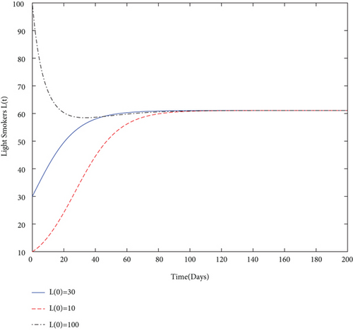
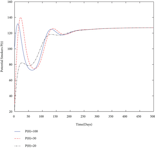
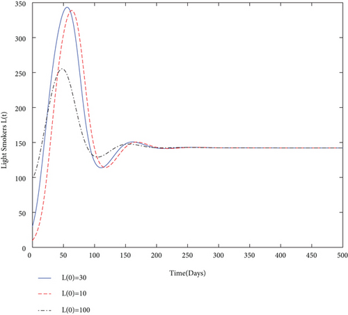
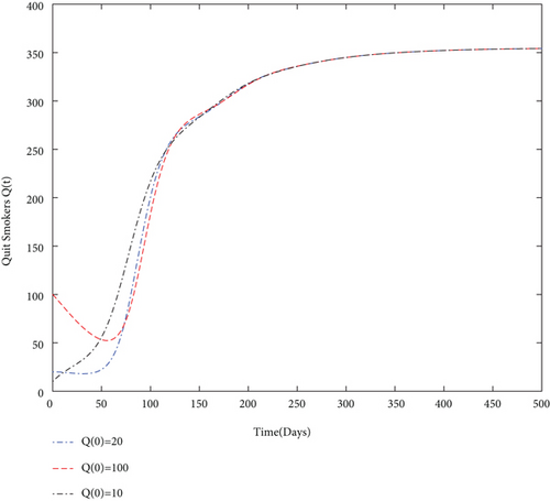
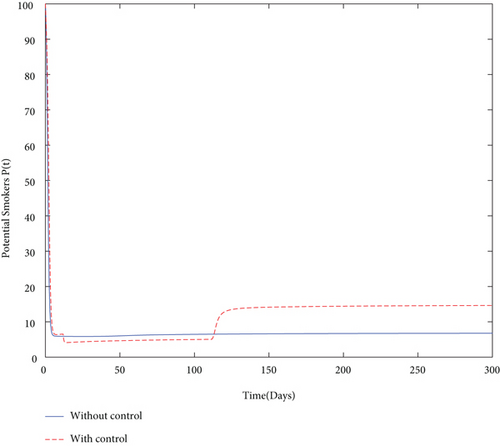
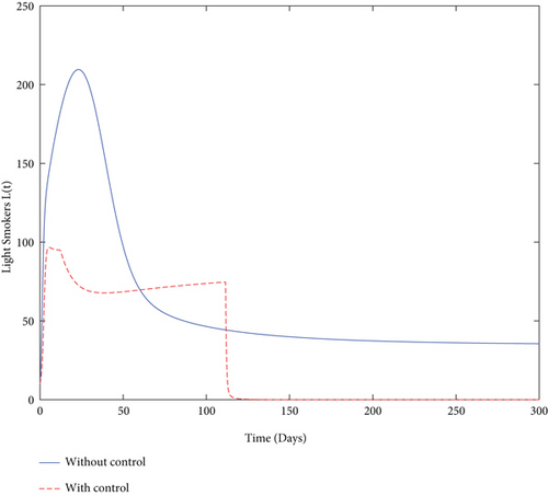
For solving the problems (both with and without controls), we used the standard RK method of fourth order. To verify numerically the key theorems on dynamical analysis, we utilized parameter values from Tables 3 and 4. Specifically, values of parameters from Table 3 were used to show the stability of smoking-free equilibrium, and sequentially, parameter values from Table 4 guarantee the stability of light smoker present equilibrium. For presenting the effect of control measures, we assumed values from Table 5. For simulating the control problem, firstly, we solved model (55) forward in time and then used backward RK4 method for solving the adjoint system (72) with the help of terminal conditions and characterization of the control variables (77)–(80). The simulation clearly illustrates the results on dynamical analysis (Figures 2 and 3) as well as on control theory (Figures 4 and 5).

Table 3. Parameter values for verifying the global stability of smoking-free equilibrium.

Parameters	Values	Parameters	Values
Λ	10.25	μ	0.08
γ	0.006	β₁	0.008
β₂	0.00038	d	0.0019
δ	0.000274

Table 4. Parameter values for verifying the global stability of light smoker present equilibrium.

Parameters	Values	Parameters	Values
Λ	10.25	μ	0.0111
γ	0.006	β₁	0.038
β₂	0.00038	d	0.0019
δ	0.041

Table 5. Parameter values are used for showing the effectiveness of the control program.

Parameters	Values	Parameters	Values
Λ	10.25	μ	0.0111
γ	0.006	β₁	0.9
β₂	0.00038	d	0.0019
δ	0.000274	q	0.2

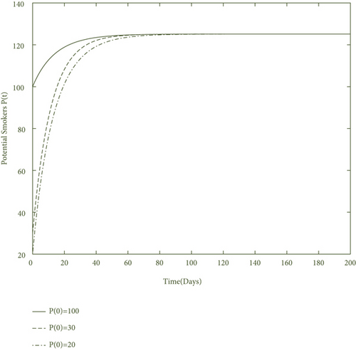
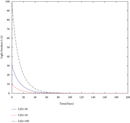
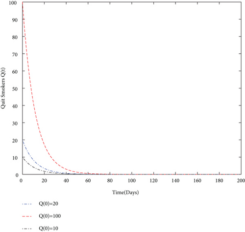
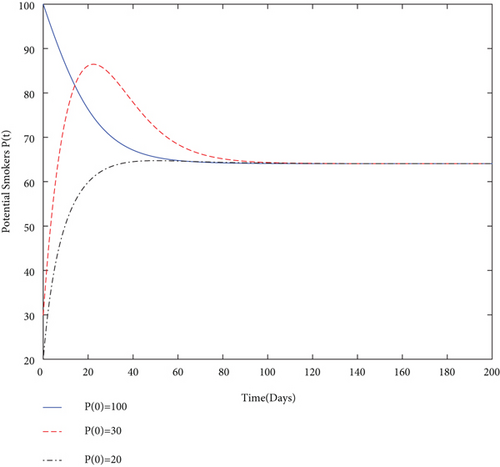
By using values of parameter from Table 3, calculate the smoking generation number R₀ = 0.1954 and SFE E₀ = (125.1526,0, 0, 0). It is clear from Figure 2 that each solution curve in the subplots tends to its SFE irrespective of the initial size of the population whenever R₀ < 1.

To show numerically the global stability of light smoker present equilibrium E_l (21), we assumed the same values of Table 3 except β₁ = 0.08 which gives R₀ = 1.9536 and as a result, E_l = (P_l, L_l, S_l, Q_l) = (64.0625,61.0901,0, 0). Thus, Figures 6(a)–6(d) shows a clear interpretation of Theorems 7 and 10, that is, if R₀ > 1, then (P, L, S, Q)⟶(P_l, L_l, S_l, Q_l) as t⟶∞.

Similarly, to show the long-term behavior of each class whenever R₀ > 1 and the side condition of Theorem 8 holds, we take into consideration values from Table 4. From these values of parameters, we calculated R₀ = 12.3077 > 1 and (P_∗, L_∗, S_∗, Q_∗) = (127,142.1,164.5,354.9). Figure 3 proves the statement of Theorem 8 as well as the global stability of SPE numerically.

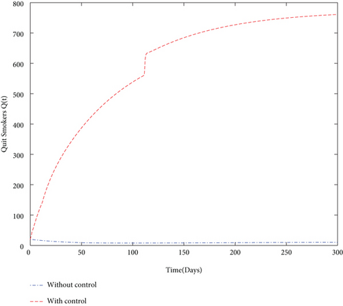
Finally, we used values from Table 5 and simulated both with and without control problems and presented the effect of the control variables. The simulation (in Figure 4) depicts in a clear way the effect of the control variables: to decrease the size of smoker population and to increase the number of quit smokers.

9. Concluding Remarks

In this work, we formulated and analyzed a giving-up smoking model utilizing three main factors related to smoking habit: the bilinear incidence rate showing the spread of smoking habit within the population from the contact of light smokers and smokers, the harmonic mean type of incidence rate (for incorporating contacts between potential smokers and occasional smokers), and the relapse factor associated to smoking. After model formulation, we investigated the model for bounded and positive solution subject to appropriate initial conditions. The model was checked for possible fixed points, and three equilibria were derived under certain conditions, namely, the smoking-free equilibrium, light smoker present equilibrium, and smoking present equilibrium. It was shown that the smoking-free fixed point always exists and is both locally and globally asymptotically stable when R₀ < 1. The positive light smoker present equilibrium exists if we assume R₀ > 1, and the same fixed point is locally as well as globally asymptotically stable if we impose additional conditions on the basic reproduction number. Further, we proved that the model has a smoking present equilibrium whenever additional conditions are satisfied by R₀. Also, a criteria for the local analysis has been derived, and the global stability of smoking present equilibrium was presented both analytically and numerically. Keeping in mind a few control measures, we set a control problem and optimal control strategies were achieved with the help of Pontryagin’s maximum principle. The obtained analytical results were verified through simulations and effectiveness of the control program is presented by comparing with and without control curves.

This work is indeed a very good contribution to the existing literature on smoking epidemics. However, this social evil has a dramatic impact on every society, and thus, one cannot ignore the memory effect while studying such and related problems. Keeping in view the importance of generalized fractional derivatives in this regard [10–30], the authors have a keen interest to formulate and analyze the fractional models for smoking epidemics in near future.

Conflicts of Interest

The author declares no conflicts of interest.

Acknowledgments

The author extends appreciation to the Deanship of Scientific Research at King Saud University for funding this work through research group no. RG-1437-017.

Open Research

Data Availability

Data availability is not applicable to this research.

References

1 Olson P. E., Hames C. S., Benenson A. S., and Genovese E. N., The Thucydides syndrome: Ebola deja vu? (or Ebola reemergent?), Emerging Infectious Diseases. (1996) 2, no. 2.
10.3201/eid0202.960220
PubMed Web of Science® Google Scholar
2 Papagrigorakis M. J., Yapijakis C., Synodinos P. N., and Baziotopoulouy-valavani E., DNA examination of ancient dental pulp incriminates typhoid fever as a probable cause of the plague of Athens, International Journal of Infectious Diseases. (2006) 10, no. 3, 206–214, https://doi.org/10.1016/j.ijid.2005.09.001, 2-s2.0-33646092772, 16412683.
10.1016/j.ijid.2005.09.001
CAS PubMed Web of Science® Google Scholar
3 Alchon S., A Pest in the Land: New World Epidemic in a Global Perspective, 2003, University of New Mexico Press.
Google Scholar
4 Rahman G. U., Agarwal R. P., and Din Q., Mathematical analysis of giving up smoking model via harmonic mean type incidence rate, Applied Mathematics and Computation. (2019) 354, 128–148, https://doi.org/10.1016/j.amc.2019.01.053, 2-s2.0-85062062745.
10.1016/j.amc.2019.01.053
Web of Science® Google Scholar
5 Kermack W. and Mckendrick A., Contributions to the mathematical theory of epidemics-I, Bulletin of Mathematical Biology. (1991) 53, no. 1-2, 33–55, 2059741.
10.1016/S0092-8240(05)80040-0
CAS PubMed Web of Science® Google Scholar
6 Hethcote H. W., The mathematics of infectious diseases, SIAM Review. (2000) 42, no. 4, 599–653, https://doi.org/10.1137/S0036144500371907, 2-s2.0-0034486891.
10.1137/S0036144500371907
Web of Science® Google Scholar
7 Kabir K. A., Kuga K., and Tanimoto J., Analysis of SIR epidemic model with information spreading of awareness, Chaos, Solitons & Fractals. (2019) 119, 118–125, https://doi.org/10.1016/j.chaos.2018.12.017, 2-s2.0-85059065777.
10.1016/j.chaos.2018.12.017
Web of Science® Google Scholar
8 Inaba H., Mathematical analysis of an age-structured SIR epidemic model with vertical transmission, Discrete & Continuous Dynamical Systems-B. (2006) 6, no. 1, 69–96, https://doi.org/10.3934/dcdsb.2006.6.69.
10.3934/dcdsb.2006.6.69
Web of Science® Google Scholar
9 Lemos-Paião A. P., Silva C. J., and Torres D. F., An epidemic model for cholera with optimal control treatment, Journal of Computational and Applied Mathematics. (2017) 318, 168–180, https://doi.org/10.1016/j.cam.2016.11.002, 2-s2.0-85008205618.
10.1016/j.cam.2016.11.002
Web of Science® Google Scholar
10 Wang X.-Y., Hattaf K., Huo H.-F., and Xiang H., Stability analysis of a delayed social epidemics model with general contact rate and its optimal control, Journal of Industrial & Management Optimization. (2016) 12, no. 4, 1267–1285, https://doi.org/10.3934/jimo.2016.12.1267, 2-s2.0-84956920356.
10.3934/jimo.2016.12.1267
Web of Science® Google Scholar
11 Hattaf K., Lashari A. A., Louartassi Y., and Yousfi N., A delayed sir epidemic model with a general incidence rate, Electronic Journal of Qualitative Theory of Differential Equations. (2013) 3, no. 3, 1–9, https://doi.org/10.14232/ejqtde.2013.1.3.
10.14232/ejqtde.2013.1.3
Google Scholar
12 Castillo-Garsow C., Jordan-Salivia G., and Herrera A. R., Mathematical models for the dynamics of tobacco use, recovery and relapse, technical report series, 1997, https://qrlssp.asu.edu/sites/default/files/mathematical_models_for_dynamics_of_tobacco_use_recovery_relapse.pdf.
Google Scholar
13 Sharomi O. and Gumel A. B., Curtailing smoking dynamics: a mathematical modeling approach, Applied Mathematics and Computation. (2008) 195, no. 2, 475–499, https://doi.org/10.1016/j.amc.2007.05.012, 2-s2.0-37349018244.
10.1016/j.amc.2007.05.012
Web of Science® Google Scholar
14 Zaman G., Qualitative behavior of giving up smoking models, Bulletin of the Malaysian Mathematical Sciences Society. (2011) 34, no. 2, 403–415.
Web of Science® Google Scholar
15 Singh J., Kumar D., Qurashi M. A., and Baleanu D., A new fractional model for giving up smoking dynamics, Advances in Difference Equations. (2017) 2017, no. 1, https://doi.org/10.1186/s13662-017-1139-9, 2-s2.0-85016157209.
10.1186/s13662-017-1139-9
Google Scholar
16 Alkhundhri Z., Al-Sheikh S., and Al-Tuwairqi S., Global dynamics of a mathematical model on smoking, International Scholarly Research Notices. (2014) 2014, 7, 847075, https://doi.org/10.1155/2014/847075.
10.1155/2014/847075
Google Scholar
17 Din Q., Ozair M., Hussain T., and Saeed U., Qualitative behavior of a smoking model, Advances in Difference Equations. (2016) 2016, no. 1, https://doi.org/10.1186/s13662-016-0830-6, 2-s2.0-84962710221.
10.1186/s13662-016-0830-6
Google Scholar
18 Rahman G. U., Agarwal R. P., Liu L., and Khan A., Threshold dynamics and optimal control of an age-structured giving up smoking model, Nonlinear Analysis: Real World Applications. (2018) 43, 96–120, https://doi.org/10.1016/j.nonrwa.2018.02.006, 2-s2.0-85042699630.
10.1016/j.nonrwa.2018.02.006
Web of Science® Google Scholar
19 Capasso V. and Serio G., A generalization of the Kermack-Mckendrick deterministic epidemic model, Mathematical Biosciences. (1978) 42, no. 1-2, 43–61, https://doi.org/10.1016/0025-5564(78)90006-8, 2-s2.0-0018041874.
10.1016/0025-5564(78)90006-8
Web of Science® Google Scholar
20 Ruan S. G. and Wang W. D., Dynamical behavior of an epidemic model with a nonlinear incidence rate, Journal of Differential Equations. (2003) 188, no. 1, 135–163, https://doi.org/10.1016/S0022-0396(02)00089-X, 2-s2.0-0037429355.
10.1016/S0022-0396(02)00089-X
Web of Science® Google Scholar
21 Mickens R. E., SIR model with square-root dynamics: an NSFD scheme, Journal of Difference Equations and Applications. (2010) 16, no. 2-3, 209–216, https://doi.org/10.1080/10236190802495311, 2-s2.0-77951180579.
10.1080/10236190802495311
Web of Science® Google Scholar
22 Zeb A., Zaman G., and Momani S., Square-root dynamics of a giving up smoking model, Applied Mathematical Modelling. (2013) 37, no. 7, 5326–5334, https://doi.org/10.1016/j.apm.2012.10.005, 2-s2.0-84872598848.
10.1016/j.apm.2012.10.005
Web of Science® Google Scholar
23 Alzaid S. S. and Alkahtani B. S. T., Asymptotic analysis of a giving up smoking model with relapse and harmonic mean type incidence rate, Results in Physics. (2021) 28, article 104437, https://doi.org/10.1016/j.rinp.2021.104437.
10.1016/j.rinp.2021.104437
Web of Science® Google Scholar
24 Mushayabasa S. and Bhunu C. P., Modelling the effects of heavy alcohol consumption on the transmission dynamics of gonorrhea, Nonlinear Dynamics. (2011) 66, no. 4, 695–706, https://doi.org/10.1007/s11071-011-9942-4, 2-s2.0-82255192990.
10.1007/s11071-011-9942-4
Web of Science® Google Scholar
25 van den Driessche P. and Watmough J., Reproduction numbers and sub-threshold endemic equilibria for compartmental models of disease transmission, Mathematical Biosciences. (2002) 180, no. 1-2, 29–48, https://doi.org/10.1016/S0025-5564(02)00108-6, 2-s2.0-0036845274, 12387915.
10.1016/S0025-5564(02)00108-6
CAS PubMed Web of Science® Google Scholar
26 LaSalle J. P., The stability of dynamical systems, 1976, Society for Industrial and Applied Mathematics.
Google Scholar
27 Tilahun G. T., Makinde O. D., and Malonza D., Co-dynamics of pneumonia and typhoid fever diseases with cost effective optimal control analysis, Applied Mathematics and Computation. (2018) 316, 438–459, https://doi.org/10.1016/j.amc.2017.07.063, 2-s2.0-85028976135.
10.1016/j.amc.2017.07.063
Web of Science® Google Scholar
28 Kamien M. I. and Schwartz N. L., Dynamic Optimization, Advanced Textbooks in Economics, 31, 1991, second edition, North-Holland Publishing Co., Amsterdam.
Google Scholar
29 Centers for Disease Control and Prevention (CDC), Best Practices for Comprehensive Tobacco Control Programs, 2015, Department of Health and Human Services, Atlanta GA.
Google Scholar
30 Hattaf K., A new generalized definition of fractional derivative with non-singular kernel, Computation. (2020) 8, no. 2, https://doi.org/10.3390/computation8020049.
10.3390/computation8020049
PubMed Web of Science® Google Scholar

All articles

Stability Analysis and Optimal Control Strategies of Giving Up Relapse Smoking Model with Bilinear and Harmonic Mean Type of Incidence Rates

Abstract

1. Introduction

2. Model Formulation and Well-Posedness

3. Equilibria of the Model and Smoker Generation Number

4. Local Stability Analysis of Equilibria

5. Global Stability Analysis of the Equilibria

6. Local Sensitivity Analysis

7. Formulation and Analysis of Optimal Control Problem

7.1. Existence of Solution to the Control Problem

7.2. Optimality Conditions

8. Simulation Results

9. Concluding Remarks

Conflicts of Interest

Acknowledgments

Open Research

Data Availability

References

Figures

References

Information

About Wiley Online Library

Help & Support

Opportunities

Connect with Wiley

Stability Analysis and Optimal Control Strategies of Giving Up Relapse Smoking Model with Bilinear and Harmonic Mean Type of Incidence Rates

Abstract

1. Introduction

2. Model Formulation and Well-Posedness

3. Equilibria of the Model and Smoker Generation Number

4. Local Stability Analysis of Equilibria

5. Global Stability Analysis of the Equilibria

6. Local Sensitivity Analysis

7. Formulation and Analysis of Optimal Control Problem

7.1. Existence of Solution to the Control Problem

7.2. Optimality Conditions

8. Simulation Results

9. Concluding Remarks

Conflicts of Interest

Acknowledgments

Open Research

Data Availability

References

Figures

References

Related

Information