Evaluation of Existing Bond-Slip Relations for CFRP-Steel Joints and New Model for Linear and Nonlinear Adhesives
Abstract
Existing bond-slip (τ-s) relations for fibre-reinforced polymer (FRP)-steel joints employ different shapes and mathematical expressions, inferring that their predictions of failure load and mode, and other interface properties, might be inconsistent or inaccurate. In this study, predictions of four widely used τ-s relations are evaluated using a large experimental database of 78 double-lap FRP-steel specimens. To facilitate the evaluation process, a robust finite element (FE) model is developed for each test, implementing data from either of the existing τ-s relations to define the FRP-steel interface. Comparisons between test and FE results indicated that the existing τ-s models were unable of predicting the ultimate load (Pu) and effective bond length (Leff) of FRP-steel joints, or the relation between Pu and bond length and that between Leff and FRP modulus (Ef). A new τ-s model is developed based on an inverse FE simulation, comparison with experimental results, and regression analysis. It considers the effects of Ef, the type of FRP reinforcement (sheet or plate), and applies to both linear and nonlinear adhesives. The model predictions were validated by comparing with results from small bond tests and large FRP-strengthened steel beams tested under bending, yielding excellent results for Pu, failure mode, and all other interfacial properties.
1. Introduction
Approximately 9% of the 614,387 bridges in the United States are designated as structurally deficient [1], of which over 52% have steel superstructures [2]. While repair and strengthening of metallic structures have historically been carried out using bolting or welding of steel plates, the use of advanced fibre-reinforced polymer (FRP) composites became a more viable alternative [2–4]. This is because of FRP’s desirable properties of high strength-to-weight ratio, corrosion resistance, and ease of transportation, handling, and installation. Of the different available FRP types, carbon-FRP (CFRP) has been heavily used in the retrofit of steel members due to its higher relative stiffness and excellent fatigue performance [2, 3]. CFRP materials are typically classified as standard modulus (SM), high modulus (HM), and ultra-high modulus (UHM) when their modulus of elasticity is less than 200 GPa, 200–400 GPa, or higher than 400 GPa, respectively [3].
Many research studies have explored experimentally the effects of strengthening or repairing steel beams and steel-concrete composite girders [3, 5–7] by adhesively bonding CFRP plates. For example, Fam et al. [3] used CFRP plates with elastic moduli varying from 200 to 400 GPa to strengthen three large-scale girders and repair 15 small-scale beams and reported 51 and 19% increase in flexural strength and stiffness, respectively, for the girders. In small beams with completely severed tension flanges, CFRP repair resulted in recovering up to 79% of strength before flange damage. Tavakkolizadeh and Saadatmanesh [5] and Al-Saidy et al. [6] also reported 44 to 76% increase in ultimate strength in composite girders strengthened with SM-CFRP and HM-CFRP plates.
In Peiris [2] and Peiris and Harik [4], UHM-CFRP strip panels were used in strengthening wide flange steel beams and single-span steel-girder bridges. Typical failure modes in SM-CFRP plates include debonding at adhesive-steel or adhesive-CFRP interfaces, cohesive failure within the adhesive layer, and CFRP delamination or rupture [3, 8]. For HM and UHM plates, rupture has been predominately reported, likely because of their lower ultimate strain and thinner section, resulting in smaller normal (peeling) and shear stresses at termination points [9]. While most research on steel strengthening has focused on SM-CFRPs, HM and UHM-CFRPs can provide better utilization of the CFRP material since they allow more load transfer to occur before yielding the steel beam [4, 8–10].
The behaviour of the strengthened member depends greatly on the effectiveness of the bonded joint in transferring loads between the steel member and FRP reinforcement and maintaining composite action, prior to desired failures. Thus, many studies were carried out on the interfacial behaviour of FRP-steel joints, mostly utilizing either single- or double-shear tests [11–15]. From these tests, an interfacial model relating the shear stress (τ) developed in the joint to the slip (s) between the two adherents is developed and presented. The τ–s relation can be used in analytical and numerical studies to evaluate the behaviour of strengthened members and assist in determining several key design results such as ultimate load, bond (development) length, and bond strength.
Several τ-s models have been suggested in previous research studies for the FRP debonding from metallic substrates [11, 16, 17]. Typically, most available models depend on the adhesive’s properties such as its tensile strength (σ_max), thickness (t_a), shear modulus (G_a), and fracture energy (G_f), and whether it is brittle (linear) or ductile (nonlinear). Although several shapes were proposed for τ-s relation, exponential and multi-linear, bilinear, and trapezoidal ones constitute the most available and widely used ones. Multiple studies deployed the empirical τ-s models in the analysis and modelling of FRP-bonded steel members.
2. Existing Bond-Slip Models
Table 1 summarizes the existing bond-slip models for CFRP-steel joints available in the literature. Although other models might also be available, those in Table 1 represent the most widely used and cited ones. These models were developed based on the results of single- or double-lap shear joints containing a steel plate bonded on one or two faces to CFRP sheets or plates. Generally, two types of models can be found in the literature, namely, bilinear models (triangle) and trilinear models (trapezoidal) (Figure 1). The difference between the two shapes is due to using either linear or nonlinear adhesive material, where the former has been reported to result in a bilinear τ–s shape and the latter to give a trilinear bond-slip shape. The following sections discuss the models developed by various researchers, their theoretical composition, strengths, and weaknesses.
| Variable | Xia and Teng [11] | Fawzia et al. [16] | Fernando [17] | Wang and Wu [18] |
|---|---|---|---|---|
| τmax | 0.8σmax | σmax | 0.9σmax | 0.9σmax |
| s1 | τmaxta/Ga | ta/10 | 0.081 mm | |
| s2 | — | — | 0.80 mm | |
| sf | 2Gf/τmax | ta/4σmax(ta = 0.1 − 0.5mm) | ||
| 0.125 + ta − 0.5/10σmaxta = 0.5 − 1.0mm | ||||
| Gf | 0.5 τmax s1 + 0.5 τmax sf (a) |
- R = tensile strain energy of adhesive, ta = adhesive thickness, Ga = adhesive shear modulus; τmax = maximum interfacial shear stress; s1 = maximum elastic slip; s2 = maximum plastic slip; sf = slip at failure; Gf = interfacial fracture energy. (a)Fracture energy represents the area under the bond-slip curve.
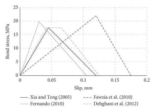
While numerous efforts have been put into developing the bond-slip relations for CFRP-steel joints, Table 1 and Figure 1 show that existing models employ different stress-slip relations and mathematical expressions, suggesting that their predictions of failure load, mode, and other interface properties might be inconsistent. This study leverages a nonlinear FE analysis and a large experimental database comprising 78 double-lap joints collected from literature to evaluate predictions of existing τ–s relations for FRP-steel joints and identify the best and worst performing ones. Based on the numerical results, a parametric study using FE simulations, and regression analysis, a new bond-slip model was developed and presented, providing much better predictions than most existing models. The model considers the effects of different parameters such as FRP modulus and type, adhesive thickness, and fracture energy and applies to both linear and nonlinear adhesives. Predictions of the proposed model have been validated by comparing with experimental results from bond and flexural beam tests.
2.1. Xia and Teng’s [11] Model
Xia and Teng [11] carried out a bond study on FRP-steel joints, using the adhesive types (A, B, and C) and four adhesive thicknesses (ta), 1, 2, 4, and 6 mm. The study proposed a bilinear relationship for the bond-slip behaviour for all adhesive types. Table 1 shows the mathematical formulation for Xia and Teng model for the key parameters, τ_max, s_1, s_2, s_f, and G_f, that define the τ–s relation. These parameters are a function of the adhesive thickness, its maximum tensile strength, and shear modulus (Table 1).
2.2. Fawzia et al.’s [16] Model
This study investigated the bond behaviour of CFRP-steel joint, using experimental and finite element results. To achieve a good understanding of the bond performance, several parameters were explored, namely, adhesive type (Sikadur 30, MBrace saturant, and Araldite 420), number of FRP layers (3 and 5), and FRP type (normal modulus and high modulus). Two values for the thickness of steel plates, 6 and 10 mm, were also investigated with a bond length ranging from 80 to 250 mm. Based on their testing and modelling protocol, the study proposed a bilinear bond-slip model, which is shown schematically in Figure 1 and a mathematical representation in Table 1. Like the previous model, the key parameters defining this model are also related to the mechanical properties of adhesive.
2.3. Fernando’s [17] Model
Fernando [17] also examined experimentally the bond-slip curve for CFRP-steel joint in terms of the effects of FRP modulus, adhesive type, and adhesive thickness. A single-shear pull-off test method was calibrated and found to be accurate for investigating the pure shear joint behaviour. The results showed that the bond strength depends significantly on the interfacial fracture energy of the adhesive layer. Nonlinear adhesives with lower moduli but larger failure strain are found to result in much higher interfacial fracture energy than linear adhesives. The shape of the τ–s model is found to be triangular and trapezoidal for Sikadur (linear) and Araldite (nonlinear) adhesives, respectively. Theoretical expressions were developed for the triangular and trapezoidal τ–s models and were used in an analytical study for predicting the full-range bond behaviour of FRP-steel joints, including estimating the effective bond length. Expressions for the trapezoidal model are shown in Table 1.
2.4. Wang and Wu’s [18] Model
Wang and Wu [18] conducted 13 single-shear tests on CFRP-steel joints and evaluated the effects of adhesive properties and thickness. They also reached the same conclusion in Fernando’s [17] study regarding the shape of τ–s model concerning adhesive type. Expressions were developed for the bilinear and trapezoidal bond-slip models for Sikadur 30 and Araldite 2015, respectively, based on fitting with the 13 experiments tested by the authors and 37 additional ones collected from the literature. The trapezoidal model by Wang and Wu is shown mathematically in Table 1, and it depends on adhesive properties, namely, σmax, ta, Ga, and the tensile strain energy of adhesive (R), which relates to the adhesive type (linear vs. nonlinear).
3. Summary of Experimental Studies
A large experimental database comprising 78 specimens was compiled in this study and used to examine the predictive capability of existing bond-slip models. To achieve this goal, a three-dimensional FE model was created for each of the test samples, implementing either of the four of the τ–s models discussed above for the steel-FRP interface.
Table 2 lists the collected test specimens, their geometric and material properties, and key experimental results. Al-Mosawe et al. [19] tested 33 double-lap of CFRP-steel specimens and evaluated the effects of FRP modulus (Ef), varying Ef from 159 to 450 GPa corresponding to three moduli (low, normal, and ultra-high), and bond length (Lf), varying Lf from 30 to 130 mm. The specimens comprise a 10 mm thick steel plate bonded to two CFRP laminates that are 1.2–1.4 mm thick (tf). The adhesive agent bonding the two adherents together was Araldite 420, a 0.5 mm thick nonlinear type. The results showed that debonding of FRP laminate was the dominant failure mode for specimens with low and normal moduli, while for those with ultra-high modulus, FRP rupture governed the behaviour.
| Ref. | Specimen ID | CFRP properties | Adhesive properties | Experimental results | ||||||
|---|---|---|---|---|---|---|---|---|---|---|
| Lf (mm) | Wf (mm) | Ef (GPa) | Tf (mm) | Ea (GPa) | Ta (mm) | Failure load (kN) | Failure mode | |||
| Al-Mosawe et al. [19] | S3-30 | 30 | 20 | 159.4 | 1.4 | 1.9 | 0.5 | 41 | DB ∗ | |
| S3-40 | 40 | 50.7 | ||||||||
| S3-50 | 50 | 60 | ||||||||
| S3-60 | 60 | 69.1 | ||||||||
| S3-70 | 70 | 76.5 | ||||||||
| S3-80 | 80 | 86.8 | ||||||||
| S3-90 | 90 | 93.6 | ||||||||
| S3-100 | 100 | 100.3 | ||||||||
| S3-110 | 110 | 108 | ||||||||
| S3-120 | 120 | 108.7 | ||||||||
| S3-130 | 130 | 109.2 | ||||||||
| NS-30 | 30 | 20 | 203 | 1.4 | 1.9 | 0.5 | 41.9 | DB | ||
| NS-40 | 40 | 51.7 | ||||||||
| NS-50 | 50 | 60.7 | ||||||||
| NS-60 | 60 | 69.8 | ||||||||
| NS-70 | 70 | 75 | ||||||||
| NS-80 | 80 | 87.4 | ||||||||
| NS-90 | 90 | 94.2 | ||||||||
| NS-100 | 100 | 101.3 | ||||||||
| NS-110 | 110 | 108.3 | ||||||||
| NS-120 | 120 | 108.5 | ||||||||
| NS-130 | 130 | 109.2 | ||||||||
| UHS-30 | 30 | 20 | 450 | 1.2 | 1.9 | 0.5 | 31.8 | DL | ||
| UHS-40 | 40 | 43.3 | ||||||||
| UHS-50 | 50 | 54.4 | ||||||||
| UHS-60 | 60 | 64.1 | ||||||||
| UHS-70 | 70 | 73.2 | R ∗ | |||||||
| UHS-80 | 80 | 73.2 | ||||||||
| UHS-90 | 90 | 73.2 | ||||||||
| UHS-100 | 100 | 73.2 | ||||||||
| UHS-110 | 110 | 73.2 | ||||||||
| UHS-120 | 120 | 73.2 | ||||||||
| UHS-130 | 130 | 73.2 | ||||||||
| Wu et al. [20] | A30 | 30 | 50 | 478.7 | 1.45 | 1.9 | 0.35 | 72.8 | DL | |
| A50 | 50 | 0.36 | 137.2 | |||||||
| A70 | 70 | 0.34 | 178.9 | |||||||
| A100 | 100 | 0.31 | 250.6 | |||||||
| A120 | 120 | 0.36 | 271.2 | |||||||
| A250 | 250 | 0.38 | 267.3 | R | ||||||
| A260 | 260 | 0.39 | 274.9 | |||||||
| Al-Zubaidy et al. [21] | CF-1-A-10 | 10 | 50 | 205 | 0.176 | 1.45 | 0.5 | 19.84 | DB | |
| CF-1-A-20 | 20 | 37.87 | ||||||||
| CF-1-A-30 | 30 | 45.22 | R | |||||||
| CF-1-A-40 | 40 | 44.06 | ||||||||
| CF-1-A-50 | 50 | 47.44 | ||||||||
| CF-1-A-60 | 60 | 46.17 | ||||||||
| CF-1-A-70 | 70 | 46.33 | ||||||||
| CF-1-A-80 | 80 | 48.18 | ||||||||
| CF-1-A-90 | 90 | 45.82 | ||||||||
| CF-1-A-100 | 100 | 46.73 | ||||||||
| CF-3-A-10 | 10 | 50 | 205 | 3 × 0.176 | 1.45 | 0.5 | 29.6 | DB | ||
| CF-3-A-20 | 20 | 54.2 | ||||||||
| CF-3-A-30 | 30 | 68.88 | ||||||||
| CF-3-A-40 | 40 | 82.88 | ||||||||
| CF-3-A-50 | 50 | 96.83 | R | |||||||
| CF-3-A-60 | 60 | 101.35 | ||||||||
| CF-3-A-70 | 70 | 103.24 | ||||||||
| CF-3-A-80 | 80 | 97.4 | ||||||||
| CF-3-A-90 | 90 | 97.38 | ||||||||
| CF-3-A-100 | 100 | 99.22 | ||||||||
| Fawzia et al. [16] | NA80 | 80 | 50 | 240 | 0.57 | 1.45 | 0.47 | 86.1 | DB/DL | |
| NA150 | 150 | 77.8 | ||||||||
| NA200 | 200 | 92.2 | ||||||||
| NA250 | 250 | 93.2 | ||||||||
| HA200 | 200 | 50 | 640 | 0.95 | 1.45 | 0.47 | 60 | R | ||
| Nguyen et al. [22] | CF1-20 | 20 | 50 | 240 | 0.18 | 1.9 | 0.5 | 33.7 | DB/DL | |
| CF1-40 | 40 | 46.5 | ||||||||
| CF1-60 | 60 | 45.5 | ||||||||
| CF1-80 | 80 | 53.1 | ||||||||
| CF3-10 | 10 | 50 | 240 | 3 × 0.18 | 1.9 | 0.5 | 29.7 | |||
| CF3-20 | 20 | 51.5 | ||||||||
| CF3-30 | 30 | 66.8 | ||||||||
| CF3-40 | 40 | 78.2 | ||||||||
| CF3-50 | 50 | 100.9 | ||||||||
| CF3-60 | 60 | 96.0 | ||||||||
| CF3-70 | 70 | 97.1 | ||||||||
| CF3-90 | 90 | 91.2 | ||||||||
| CF3-100 | 100 | 98.2 | ||||||||
- ∗DB = FRP debonding; DL = FRP delamination; R = FRP rupture.
Wu et al. [20] also conducted double-lap tests to investigate the behaviour of CFRP-steel bonded joints. UHM-CFRP laminates, with an Ef = 460 GPa and tf = 1.45 mm, were used and were bonded to steel using two types of adhesive, Araldite 420 and Sikadur 30. The study evaluated the effects of adhesive properties, bond length, and laminate thickness as listed in Table 2. The study reported that FRP delamination or rupture was the governing failure mode in specimens with Araldite 420 adhesive compared with debonding failure (hereafter debonding failure referring to interface failure) for those with Sikadur adhesive. Also, Araldite 402 helped to achieve higher strength due to its much larger elongation deformation at break compared with Sikadur adhesive. It should be noted that only specimens bonded with Araldite 420 are presented in Table 2.
The third group in Table 2 is the 20 quasi-static double-lap specimens tested by Al-Zubaidy et al. [21]. The primary variables were Lf (bond length), which varied from 10 to 100 mm, and several FRP layers, either one or three. The study revealed that an increasing number of FRP plies contributed to increasing joint strength. Observed failures were FRP debonding for lengths shorter than the effective bond length (Leff) and FRP rupture when Lf was longer. Leff was estimated to be 30 and 50 mm for 1 ply and 3 FRP plies, respectively. Fawzia et al. [16] also tested several adhesively bonded double-lap joints and studied the effects of Lf for normal (Ef = 240 GPa) and high (Ef = 640 GPa) modulus CFRP, varying Lf from 80 to 250 mm, and thickness of steel plate. The results showed a mixture of failure modes, with debonding and FRP delamination as the dominant ones. Nguyen et al. [22] also performed experiments on a series of FRP-steel bond specimens using one and three FRP layers and a wide range of bond lengths (Table 2).
4. Finite Element Modelling
The general purpose ABAQUS software V6.16 [34] was used in this study to examine the numerical response of FRP-steel interfaces and bond-slip models presented in Section 2. The explicit solver was selected due to its efficiency and capability of overcoming convergence problems particularly when contact or highly nonlinear behaviour is present. Each model imitated the geometric and material properties of the specimens in Table 2, as they were given in the experimental references.
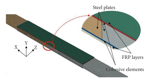
Due to the symmetry of the double-lap joint in terms of material, loading, and geometry and to reduce computational work, only one-eighth of the full-size specimen was modelled. At the respective planes of symmetry, proper translational and rotational constraints were imposed. The model was fixed by imposing translational longitudinal constraints into the CFRP plate and loaded by applying an incremental longitudinal displacement into the steel plate. A mesh sensitivity study was conducted to choose the optimal mesh size using several sizes including 5, 2, 1, and 0.5 mm. This was conducted for the bond region, while the rest of the specimens had a 5 mm mesh size. A fine mesh, with a maximum element length of 1 mm, was used for all parts (steel, FRP, cohesive elements) inside the bonded region and was gradually increased to 5 mm long elements for other regions (Figure 2). The adhesive layer was modelled by cohesive elements, which were bonded to the steel or FRP parts by master-slave contact, assuming the adhesive layer is the slave entity, and the latter two parts are the master entity.
4.1. Element Selection
The FRP-steel joint consists of three main parts: steel, adhesive, and FRP. Among the different elements that are available in ABAQUS, appropriate ones have been selected for each part depending on the recommendations of previous studies conducted on similar joints [8, 13, 23]. Solid elements C3D8R were employed in the modelling of the steel plate. Linear three-dimensional four-node shell elements S4R with reduced integration were used for modelling FRP, while eight-node three-dimensional cohesive elements, COH3D8, were used in modelling the adhesive layer.
4.2. Material Modelling
4.2.1. Steel
A linear elastic material model was selected for the steel part, using an elastic modulus (Es) of 200 GPa and Poisson’s ratio (v) of 0.3. This model was used because, in all experimental specimens in Table 2, the steel plate was behaving elastically and did not experience yielding or permanent deformations. In addition, the value of elastic modulus was assumed since, in most of the simulated experimental studies, the elastic modulus of steel was not provided.
4.2.2. CFRP
Like most unidirectional FRP composites simulated in ABAQUS [24], the CFRP plate/sheet was modelled as an orthotropic lamina with linear elastic properties. The FRP rupture failure that occurred in several specimens, particularly those with bond lengths greater than Leff, is explicitly simulated in this study, using Hashin’s failure criteria [25].
4.2.3. Cohesive Zone Material
- (1)
Elastic stage: during the first elastic region (segment O-A in Figure 3), stress increases linearly with displacement until the damage initiation criterion is activated when the stress reaches the prescribed strength value. The moduli for the elastic portion are defined by three stiffness values, Knn, Kss, and Ktt, which can be calculated as follows:
(1)(2)where Knn, Kss, and Ktt are the elastic stiffness values for the normal and two shear directions, respectively; Ea and Ga are Young’s and shear moduli for the adhesive layer, respectively; and ta is the thickness of the cohesive element (or adhesive layer). For the specimens in Table 2, Ea, Ga, and ta were taken from the experimental reference corresponding to each sample. - (2)
Damage initiation criteria: the damage criterion is a quadratic stress failure expression (QUADSCRT), which considers the mixed mode, normal (mode I) and shear (mode II) of failure. It is assumed that the damage is initiated when the following equation is satisfied:
(3)where tn, ts, and tt are the stresses in three orthotropic directions in the adhesive layer, and , , and are the adhesive strengths in the same respective axes. - (3)
Damage evolution law: once the damage initiation occurs, the last stage (damage evolution) begins signalling cumulative degradation in the stiffnesses of the cohesive elements and progression of debonding. This stage is represented by line AC for the bilinear model or by the two lines AB and BC for the trilinear model (Figure 3).
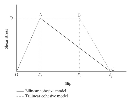
Since there are only three traction-separation laws available in ABAQUS, which are the bilinear, exponential, and tabular traction-separation laws, therefore the trilinear (trapezoidal) bond-slip models, such as Fernando [17] and Wang and Wu [18], cannot be implemented directly into ABAQUS. However, the tabular cohesive model functionality can be used to implement the damage variable (D) for the trilinear law.
5. Predictions of Existing Models
FE analysis was conducted for each of the 78 experimental samples in Table 2 to examine the accuracy of the four bond-slip models discussed in Section 2 in simulating the bond behaviour of FRP-steel joints. In implementing the FE model for evaluation purposes, the inputs required for the traction-separation law, for example, tno, tso, tto, and sm, were obtained from the theoretical expressions associated with each of the examined τ–s models in Table 1. Figure 4 plots the ultimate load (Pu) comparisons from either test results or predictions of FE simulations implementing the four examined τ–s models.
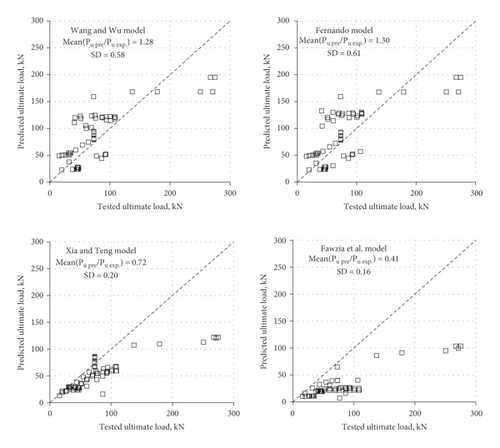
FE analysis was conducted for each of the 78 experimental samples in Table 2 to examine the accuracy of the four bond-slip models discussed in Section 2 in simulating the bond behaviour of FRP-steel joints. In implementing the FE model for evaluation purposes, the inputs required for the traction-separation law, for example, , , , and sm, were obtained from the theoretical expressions associated with each of the examined τ–s models in Table 1. Figure 4 plots the ultimate load (Pu) comparisons from either test results or predictions of FE simulations implementing the four examined τ–s models.
The existing models provided a prediction of Pmax with various levels of accuracy compared with experimental results, when the mean value of predicted/tested Pu was 0.72, 0.41, 1.30, and 1.28 for the models by Xia and Teng [11], Fawzia et al. [16], Fernando [17], and Wang and Wu [18], respectively. Also, the models by Xia and Teng [11] and Fawzia et al. [16] generally underestimated Pu, while those by Fernando [17] and Wang and Wu [18] provided over predictions of Pu, but at much better accuracy. In terms of failure mode, the numerical specimens corresponding to Xia and Teng [11] and Fawzia et al.’s [16] τ–s models failed mostly by debonding, while those containing Fernando [17] and Wang and Wu’s [18] expressions failed predominantly by FRP rupture. These results are contrary to the failures reported experimentally, namely, debonding, if Lf is shorter than Leff, or rupture and/or cohesive otherwise. The numerical trend can be attributed to the relatively high fracture energy of the trapezoidal models by Fernando [17] and Wang and Wu [18] (Figure 1), which allow for more stress transfer from steel to FRP to occur, delaying debonding and promoting rupture, in contrast to the other two bilinear models with low fracture energy.
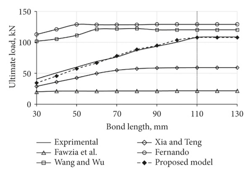
Figure 5 plots the relation between Pu and Lf, as obtained from test results from Al-Mosawe et al. [19] study or FE predictions using either of the τ–s models. The existing models provided some differences from the experimental results regarding Pu and Lf relation or predict the effective bond length (Leff). The Pu values corresponding to Fernando [17] and Wang and Wu [18] bond-slip models were overly predicting test results, particularly for short bond lengths. On the contrary, Xia and Teng [11] and Fawzia et al.’s [16] τ–s models yielded severe under predictions, particularly at longer bond lengths.
- (1)
The diverging results from existing τ–s models necessitate the development of a new bond-slip model capable of yielding better predictions for a range of material and geometric variations.
- (2)
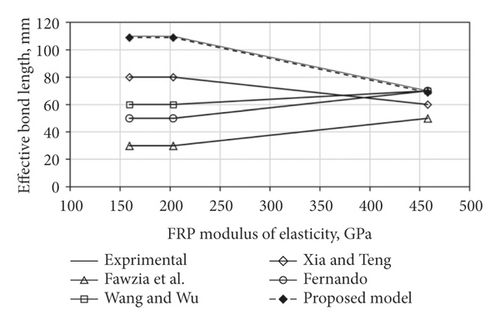
Some studies [19] found that the effective bond length is significantly affected by Ef, yet none of the existing bond-slip models considers this parameter.
- (3)
Existing τ–s models do not distinguish between FRP laminate (plate) and sheet. Since laminates have a larger shear deformation capacity than sheets [20], this parameter also needs further evaluation.
6. Proposed Model
In this section, a new τ–s model is proposed, aiming at overcoming the limitations of the existing models discussed earlier and providing better predictions for the interfacial behaviour of FRP-steel joints. The model was developed using a hybrid procedure that relies on experimental results, FE models, regression analysis, findings, and recommendations from literature. In utilizing the test results of Table 2, only specimens failing by debonding or cohesions were included in model development. These specimens were modelled numerically, and an inverse analysis (shown graphically in Figure 7) was implemented where for each specimen, the FE load step corresponding to Pmax from experimental results is used to extract fracture energy for the FRP-steel joint and evaluate the effects of several key variables.
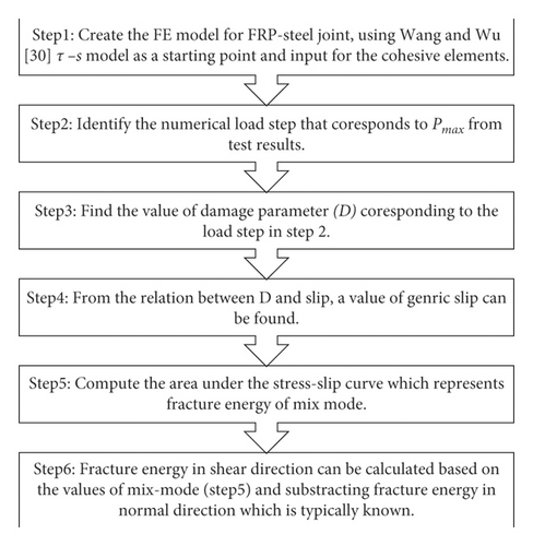
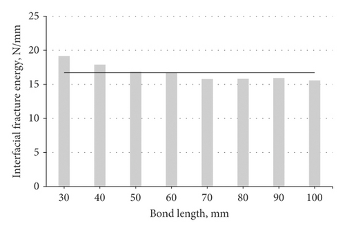
Figure 8 plots the interfacial fracture energies (Gf) for several specimens in Al-Mosawe et al. [19] tests, extracted from the inverse analysis procedure, against the bond length. Gf is approximately constant across different lengths, with an average value of 17 N/mm. Furthermore, multiple studies classified Gf into two groups based on the FRP type whether it is laminate or sheet [17, 20]. For instance, Wu et al. [20] found that Leff of joints with FRP laminates was longer than that with FRP sheets, likely because the former has a larger shear deformation capacity than the latter and is thicker.
6.1. Effects of FRP Modulus on Gf
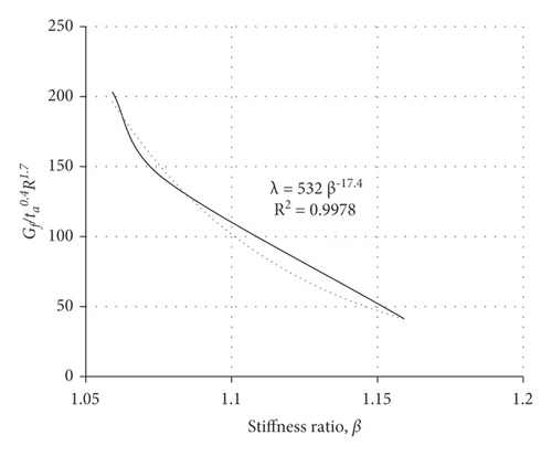
The effect of β can be quantified by plotting the term Gf/ta 0.4R1.7 versus β for different FRP types as shown in Figure 9. Based on curve-fitting analysis of the results of Figure 9, (10) can be rewritten as in equation (13).
6.2. Effects of FRP Types on Gf
6.3. Peak Shear Stress
Analysis of experimental results and trends in Table 1 show that the peak shear stress (τmax) in existing bond-slip models is unanimously related to adhesive properties, while its value only varies by a small percentage from 1 to 0.8 the adhesive tensile strength (σmax). An average value of 0.9σmax is suggested in this study for τmax, following the recommendations of [13, 16, 17] who conducted relatively large experimental campaigns compared with those in other studies.
6.4. Interfacial Slip
As shown in Figure 3, the interfacial slip (s) is defined by three points: (1) the maximum elastic slip (s1) at τmax, where s1 applies to both the bilinear and trapezoidal models; (2) the maximum plastic slip (s2) also at τmax for the trapezoidal model; and (3) and the slip at debonding completion (sf) or when τ = 0, applicable to both models. The following subsections discuss the proposed expressions for s1, s2, and sf.
6.4.1. Maximum Elastic Slip (s1)
6.4.2. Maximum Plastic Slip and Slip at Failure
Significant variation for the values of s2 and sf can be noticed in predictions from existing τ–s models. For instance, when these values are calculated for the specimens tested by Al-Mosawe et al. [19], they are ranged between 0.61 to 0.8 mm and 0.125 to 2.11 mm for s2 and sf, respectively. It can be concluded from Tables 1 and 3 that the ratio of sf/s2 was 2.0 for Wang and Wu’s [18] τ–s model and is variable in Fernando's [17] model. In addition, the research by Dehghani et al. [26], which also discussed the bond-slip behaviour of steel-FRP joints, proposed a value of 3 for sf/s2 ratio.
| Bond-slip model | Gf (N/mm) | s2 (mm) | sf (mm) | sf/s2 | |
|---|---|---|---|---|---|
| Xia and Teng [11] (triangular model) | 4.20 | — | 0.36 | — | |
| Fawzia et al. [16] (triangular model) | 0.46 | — | 0.125 | — | |
| Fernando [17] (trapezoidal model) | 37.1 | 0.80 | 2.11 | 2.6 | |
| Wang and Wu [18] (trapezoidal model) | 22.3 | 0.61 | 1.22 | 2.0 | |
| Proposed model | FRP-low modulus | 17.6 | 0.36 | 0.90 | 2.5 |
| FRP-normal modulus | 11.4 | 0.23 | 0.58 | 2.5 | |
| FRP-UH modulus | 3.5 | 0.08 | 0.19 | 2.5 | |
- ∗ Gf = interfacial fracture energy; sf = slip at failure; s2 = maximum plastic slip.
7. Evaluation of the Proposed Model
In this section, the predictability of the proposed model (τmax = 0.9 σmax, Equations (14)–(16)) is evaluated by implementing the model into FE analysis of FRP-steel joints and comparing the numerical results with those from experiments, a process identical to that undertaken in Section 5. To provide accurate and unbiased evaluations, the majority of experimental specimens used in this section for testing the predictability of the proposed model were different from those used in previous sections for model development. The differences were in FRP width, adhesive thickness, FRP lengths, and FRP properties. The following subsections discuss various results obtained from the model and comparisons with test data, showing the model’s ability to capture the behaviour of FRP-steel joints.
7.1. Ultimate Load
Figure 10 plots the ultimate load (Pu) comparisons from either test results or predictions of FE simulations implementing the proposed τ–s model. It can be seen clearly that the predicted and test values of Pu are in good agreement, where the mean value of predicted (Pu pre)/experimental (Pu exp) ultimate loads is 1.01 with a standard deviation of 0.078. Compared with the Wang and Wu’s [18] model, which was the best performing among the four existing models with a (Pu pre)/(Pu exp) of 1.28 and a standard deviation of 0.58 (Figure 4), the proposed model yielded much better predictions, reflecting a higher level of accuracy.
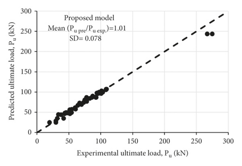
Figure 5 plots the relation between Pu and FRP-bond length (Lf) and shows that the proposed model can capture the variation of Pu with Lf, with a good level of accuracy. The model resulted in an effective bond length (Leff) of 110 mm, which is identical to that reported in experiments. Figure 6 shows the relation between Leff and FRP modulus (Ef), where Leff is determined from test results or FE simulations corresponding to existing models and the proposed one. It can be seen from the figure that the proposed model is able of predicting the variation of Leff concerning various FRP modules (low, normal, high, ultra-high).
7.2. CFRP Strain Distribution
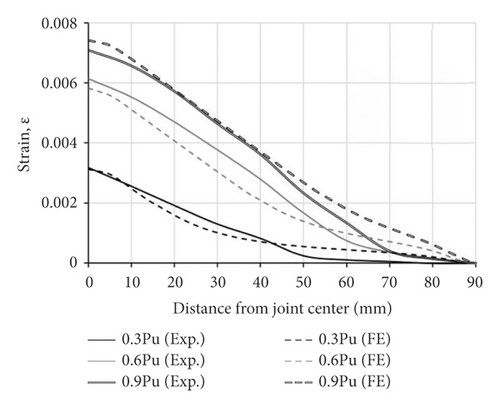
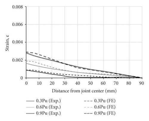
The bond-slip model affects the forces transferred from steel to FRP and ultimately the strains developed in the composite material. It is therefore necessary to also test the model predictions in terms of FRP strains. Figure 11 plots two representative double-lap specimens and the strains along the bond length of CFRP laminate, comparing results from the test and those from FE simulations using the proposed τ–s model. Figure 11 shows the model’s ability to simulate the FRP strains at various loading levels and in different locations along with Lf, for two different FRP moduli, low in specimen NS-90 and ultra-high in specimen UHS-90.
7.3. Load-Slip Curve
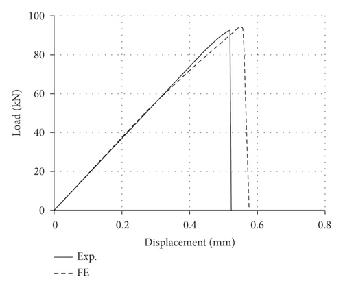
The load-joint displacement (P-Δ) response provides other means of validating the predictions of the proposed bond-slip model. Figure 12 presents the P-Δ comparisons from testing and the FE model corresponding to the proposed τ–s model, for a representative specimen CF3-BL100 from Table 2. The FE-based P-Δ agreed well with that from the experiment in terms of stiffness and ultimate load, with a slightly larger, 0.57 vs. 052 mm, Δ at ultimate.
7.4. Mode of Failure
A robust bond-slip model must be able to yield similar failure modes to those observed experimentally. Figure 13 shows the FE failure progression in three representative specimens from Table 2, NS-50, NS-70, and UHS-80, from experiments and FE model corresponding to the proposed τ–s model. Figure 13(a) plots the experimental and numerical damage parameters in relation to joint displacement and shows the model’s ability to trace the debonding failure along the loading path. In this figure, three points along the numerical damage parameter-displacement curve are indicated, point 1 (at no debonding), point 2 (moderate debonding), and point 3 (complete debonding).
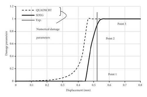
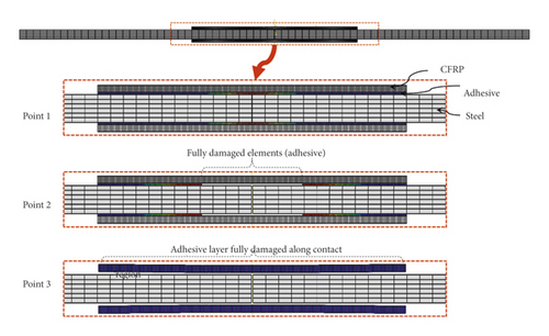
The FE model corresponding to either of these three points is given in Figure 13(b), showing the physical debonding in the adhesive layer. Overall, the proposed model demonstrated a good correlation with test results, a reasonable variation with different key parameters, and superior performance compared with existing models. However, further research must be conducted to validate the model’s predictions with a larger and more diverse experimental database and to carefully study the effects of two parameters found in this study to impact the τ–s model, namely, FRP type (sheet vs. laminate) and FRP modulus.
8. Beam Case Studies
In previous sections, the proposed τ–s model is evaluated against experimental results of small-scale steel-FRP joints. In this section, the model is validated against large-scale FRP-bonded beam tests, which are more realistic and representative of field applications than single- and double-lap specimens. Two sets of beam tests are used in the validation procedure and are detailed in the following subsections. The same modelling methodology (element types, constitutive relations, loading type, etc.) that was used for the double-lap joints and discussed in previous sections is implemented herewith for the beam models.
8.1. Deng and Lee’s [27] Tests
In this experimental work, three steel beams with a length of 1.2 m and a 127 × 76 UB13 section were strengthened with 3 mm thick CFRP plates and tested in flexure to failure, under three points. The primary variable in the testing campaign was the CFRP length, ranging from 300 to 500 mm, as shown in Table 3. A normal modulus, Ef = 212 GPa, CFRP plate was used in the tests. The adhesive material used to bond the CFRP plate to the beam soffit was Sikadur 31 (linear type), whose properties and inputs are given in Table 4.
| Specimen ID(1) | L(2) (mm) | Pu(2) (kN) | Δu(2) (mm) | Failure mode | |||||
|---|---|---|---|---|---|---|---|---|---|
| Exp. | FE | % | Exp. | FE | % | Exp. | FE | ||
| S3031 | 300 | 120.0 | 121.2 | 1.0 | 5.12 | 4.68 | 9.4 | DB 3 | DB |
| S3041 | 400 | 135.0 | 134.8 | 0.1 | 7.00 | 7.71 | 9.2 | DB | DB |
| S3051 | 500 | 149.1 | 141.9 | 5.1 | 12.43 | 11.51 | 8.0 | DB | DB |
| B501 | 500 | 93.7 | 97.1 | 3.5 | -- | 8.67 | -- | DB | DB |
| B651 | 650 | 105.9 | 106.6 | 0.7 | 10.06 | 9.44 | 6.6 | DB | DB |
| B1201 | 1200 | 143.0 | 148.0 | 3.4 | 19.39 | 19.52 | 0.7 | R 3 | R |
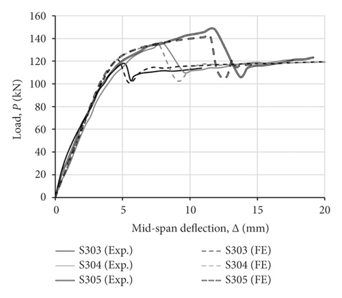
Figure 14(a) plots the load (P) versus mid-span deflection (Δ) curves for the three tested beams and three corresponding FE models using the proposed τ–s model. The general P-Δ response from the FE models is in very good correlation with test results, and the model was able to simulate the pre- and post-yielding stiffness for each beam. The ultimate load (Pu) ratio, numerical/experimental (Pu FE/Pu Exp), varied from 5.12 to 12.43%, with an average value of 8.18% for all three beams. Similarly, the numerical/experimental ratio for the deflection at ultimate was less than 10% for all beams. The failure mode observed in tests was debonding of the CFRP laminate and was accurately simulated in the FE models, reflecting excellent correlations from the proposed τ–s model.
8.2. Lenwari et al.’s [28] Study
This study tested three steel beams, with a span of 1.8 m and a W100 × 17.2 section, strengthened in flexure by three different CFRP lengths as listed in Table 3. Steel plates, having 200 mm width and 12.2 mm thickness, were welded to the top flange of the steel beams to prevent compressive yielding. A high modulus, Ef = 300 GPa, CFRP plate with an ultimate strength of 1400 MPa was used in the study. The bonding agent between CFRP and steel was Sikadur 30 (linear type), whose properties and inputs are given in Table 4.
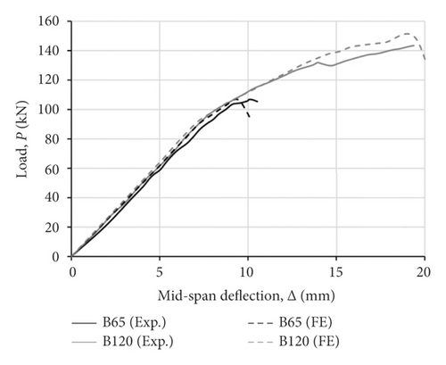
Figure 14(b) plots P-Δ curves for the three tested beams and three corresponding FE models using the proposed τ–s model. Like the previous tests in [27], the FE models simulated accurately the general P-Δ response and stiffness for beams B50, B65, and B120 from Lenwari et al.’s [28] study. The maximum (Pu FE/Pu Exp) ratio was less than 3.5%, indicating a close correlation for the ultimate load. The FRP rupture and debonding failures reported in [28] were both captured by the FE models. The combined results from the 6 beam specimens tested by [27, 28] confirm the capability of the proposed τ–s model to accurately represent the FRP-steel interface, leading to excellent predictions for the flexural behaviour of FRP-bond steel.
9. Conclusions
- (i)
None of the existing models was able to provide a good prediction for the ultimate load (Pu) and effective bond length (Leff) of FRP-steel joints. The ratio between predicted and tested Pu ranged from 0.41 to 1.3 with large standard deviations.
- (ii)
A new τ-s model is proposed and considers the effects of several parameters not included in existing models, namely, FRP modulus (Ef), ranging from normal to ultra-high modulus, and type of FRP reinforcement (sheet versus plate). The model takes a trapezoidal shape and applies to both linear and nonlinear adhesives.
- (iii)
Predictions of the proposed model were validated by comparing with results of double-lap joint tests, yielding excellent predictions for Pu, FRP strains, and failure modes. Unlike other τ-s expressions, the proposed model was able to capture the relation between Pu and bond length and that between Leff and Ef.
- (iv)
Full-scale bending tests were also deployed to confirm the accuracy of the proposed τ-s model for actual FRP-strengthened members. The model resulted from inaccurate predictions of ultimate load, load-deflection curves, and failure modes for 6 simulated beams with different strengthening lengths, Ef, and adhesive types.
Disclosure
The research was performed as part of the employment of the authors. These include (i) University of Babylon, Hilla, Iraq; (ii) Queen’s University, Kingston, Canada; (iii) Al-Mustaqbal University College, 51001, Babylon, Iraq; and (iv) Lulea University of Technology, Lulea 97187, Sweden.
Conflicts of Interest
The authors declare no conflicts of interest.
Open Research
Data Availability
All data are included within the article.


