Support vector regression (SVR) has been applied to the prediction of mechanical properties of concrete, but the selection of its hyperparameters has been a key factor affecting the prediction accuracy. To this end, hybrid machine learning combines the SVR model and grid search (GS), namely, the GS-SVR model was proposed to predict the compressive strength of concrete and sensitivity analysis in this work. The hybrid model was trained and tested on a total of 98 datasets retrieved from literature, and the model performance was compared with the original SVR model under the same datasets. The obtained results in terms of R of 0.981, MSE of 3.44, RMSE of 1.85, MAE of 1.17, and MAPE of 0.05 demonstrate that the GS-SVR model proposed can be a candidate method for compressive strength prediction in subsequent related studies. Additionally, a graphical user interface (GUI) was developed to conveniently provide some initial estimates of the outcomes before performing extensive laboratory or fieldwork. Finally, the effect of each variable on the compressive strength in a random environment was analyzed.

1. Introduction

As the most consumed material in the construction industry, cement has brought great convenience to the construction industry. But the bad news is that it also puts enormous pressure on the environment. Since the production and utilization of cement are accompanied by a large amount of greenhouse gas emissions, many scholars have started to focus on research related to mineral admixtures that can be used to replace cement [1–5]. Among them, the use of fly ash as an auxiliary cementitious material for the production of a large amount of fly ash concrete is one of the important ways to reduce environmental pollution and realize the resourcefulness of fly ash. Moreover, it is also an effective means for concrete producers to enhance and improve the performance of concrete in all aspects, reduce the use of cement, and lower the cost of concrete [6, 7]. The incorporation of fly ash not only ensures the quality of concrete and reduces the cost of manufacturing concrete but also improves the compatibility, durability, and strength, thus becoming the most widely used alternative and receiving great attention [8].

The importance of concrete materials for the construction industry needs no more introduction [9–11]. Concrete is used as a construction material worldwide due to its various properties such as strength, durability, stiffness, and fire resistance. Among these properties, compressive strength is considered to be the most important one because it seriously affects the safety and durability of concrete members. Understanding the early behavior of concrete allows appropriate measures to be taken to avoid problems such as cracking and deformation of concrete members, formwork failure, and rework. In addition, early strength prediction and monitoring are important for assessing construction safety, determining structural maturity, and predicting later strength development. The main reason for different compressive strength values of concrete is that concrete is a nonhomogeneous material consisting of binders, aggregates, water, and admixtures. In such a complex mix, it is difficult to find or predict the compressive strength of concrete accurately. The compressive strength of concrete can be assessed in the laboratory by crushing a standard size cylinder or cube. However, such laboratory tests are supposed to be inefficient and uneconomical, as well as labor-intensive and time-consuming. Traditional methods of concrete strength prediction are mainly based on a statistical analysis of linear or nonlinear regression equations, but obtaining accurate equations is difficult and requires a great deal of skill and experience. Due to the large number of concrete ingredients, it seems difficult to establish an explicit equation between the compressive strength and each ingredient as a way to predict its compressive strength.

To address these issues, machine learning techniques are used to predict the compressive strength of concrete. In fact, with the development of artificial intelligence, various machine learning algorithms such as artificial neural network (ANN), support vector machines (SVM), random forest, and extreme learning machine (ELM) have been applied to predict the mechanical properties of concrete [12–23]. Ly et al. [24] employed an optimal deep neural network model on a database of 223 experimental data to predict the 28 days compressive strength of rubber concrete and achieved a high prediction accuracy of R = 0.9874. Han et al. [25] utilized an optimized random forest approach on 1030 data samples collected from published literature to predict the compressive strength of high-performance concrete. Furqan et al. [26] used the ANN, SVM, and gene expression programming (GEP) on 300 datasets to predict the compressive strength of self-compacting concrete. Zhang et al. [27] employed nine machine learning models to predict the compressive strength of concrete at the age of 7 days and found that the nonlinear models had better predictive performance than the linear models. Khoa et al. [28] employed deep neural networks (DNNs) and ResNet models for compressive strength prediction of green fly ash-based geopolymer concrete. The results showed that ResNet is superior and indicated that these two machine learning methods can be useful for the mixed design of geopolymer concrete. From the published studies, it can be found that these machine learning algorithms outperform traditional empirical formulations by enabling the capture and mapping of multidimensional nonlinear relationships. It is possible to extract unknown relationships and data information between input and output variables [29].

However, these models also have limitations, and many models require parameter tuning to get better performance. For support vector regression (SVR), the selection of hyperparameters has a great impact on the accuracy of the prediction results. In other words, the prediction accuracy of a single SVR model is limited. To better understand and apply the SVR method, further exploration is still needed in this area using different datasets and optimization algorithms. For this reason, this study aims to propose a hybrid machine learning that combines the SVR model and grid search (GS), namely, the GS-SVR model, to achieve an accurate prediction of the compressive strength of fly ash concrete. Based on the model, the effect of random variation of individual variables on compressive strength is investigated as a reference and guide for concrete mix design and strength prediction.

2. Methodology

2.1. Support Vector Regression

The objective of the SVR is to find a linear regression equation that fits all sample points and minimizes the total variance of the sample points from this regression hyperplane. There is a sample training set E = {(x_i, y_i)|i = 1,2, …n}, x_i ∈ Rⁿ, y_i ∈ R. A function f (x_i) is probed on Rⁿ, such that y_i = f (x_i), and there is always a corresponding y-value for any input x. Such a function f (x_i) is called a regression function, and f (x_i) can be described as follows.

(1)

where ω ∈ Rⁿ is the weight vector, ϕ(x_i) is a nonlinear mapping which serves to map the data from the space Rⁿ to the higher feature space, and b is the bias. Equation (1) can be fitted to all sample points at precision ε.

(2)

Since there is a certain fitting error, the slack variables (ξ_i, ξ_i ^∗) and the penalty parameter C are introduced. The regression fitting problem is changed to an optimization problem.

(3)

Using Lagrange multipliers for equation (3), the Lagrange function is introduced to obtain its dual form.

(4)

The core of optimization at this point is to first determine the feature space and find the flattest function in that space that satisfies the conditions and then use that function to solve the nonlinear problem. For this reason, the kernel function K(x_i, x_j), K(x_i, x_j) = ϕ(x_i) · ϕ(x_j) is introduced. The regression fitting function at this point is

(5)

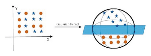
There are many choices of kernel functions, and the commonly used RBF function (Figure 1) is chosen in this study [30].

Details are in the caption following the image — Open in figure viewer PowerPoint

2.2. Grid Search Method

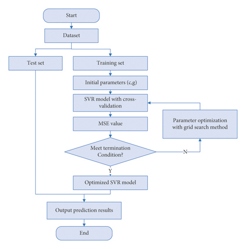
It is well known that the identification results depend heavily on the selection of hyperparameters of the SVR model. Since the parameters are highly nonlinear, a large number of experiments are often required to determine the combination of parameters, such as the penalty parameter C and the kernel parameter g. Although Lin et al. [31, 32] have done much extensive research to simplify the application of SVM, such as proposing LIBSVM, the selection of parameters C and g still depends on experience. Therefore, there is an urgent need to implement automatic tuning of parameters to obtain the optimal value once the parameters are entered. The grid search (GS) method can solve these problems. The GS method is to computationally evaluate the impact of each parameter combination on the model performance by iterating through all the candidate parameter choices in a loop to obtain the optimal combination of hyperparameters [33]. The flowchart of parameter selection is shown in Figure 2.

3. Dataset Description

3.1. Input and Output Variables

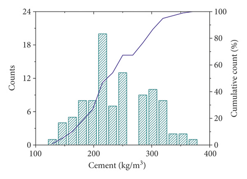
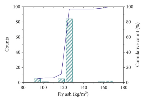
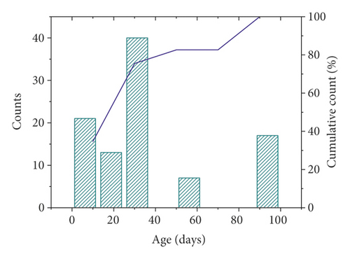
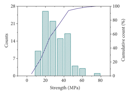
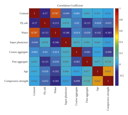
In this study, 98 sets of data were retrieved from the literature. Each dataset consisted of six constituents (cement, fly ash, water, super, plasticizer, coarse aggregate, and fine aggregate) and age as input variables and the compressive strength as output variable. The distribution of the input and output variables is shown in Figure 3, and the statistical characteristics of these variables are given in Table 1. It can be seen that the compressive strength varies greatly for different combinations of input variables. Additionally, Pearson correlation coefficients between input and output variables were plotted, as shown in Figure 4. Within the current dataset, linear correlation between any of the input and output variables is weak, which indicates a complex nonlinear relationship between compressive strength and these input parameters. Therefore, the relationship between compressive strength and these parameters is difficult to reflect by an explicit equation.

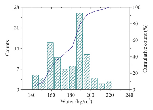
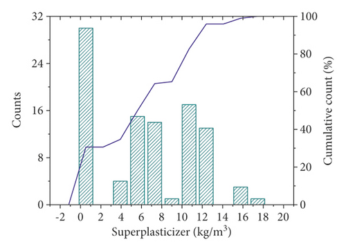
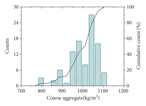
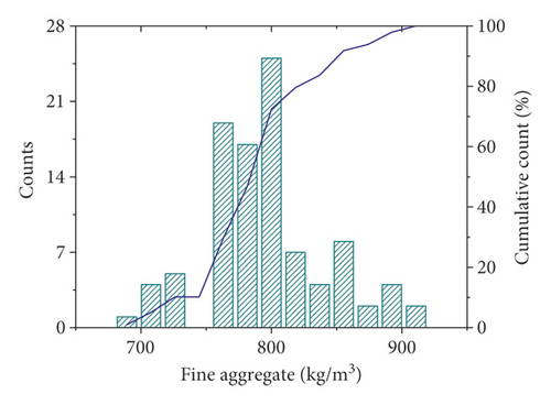
1. Statistical characteristics of variables.

		Cement	Fly ash	Water	Super plasticizer	Coarse aggregate	Fine aggregate	Age	Compressive strength
Training set	Unit	kg/m³	kg/m³	kg/m³	kg/m³	kg/m³	kg/m³	d	MPa
	Count	78	78	78	78	78	78	78	78
	Maximum	376	163.3	216.7	18	1118	905.4	90	72.11
	Minimum	136.1	92.1	141.1	0	801	700	3	9.49
	Standard deviation	54.22	9.68	18.12	4.65	67.60	44.70	29.72	13.37
	Mean	243.95	123.54	177.77	6.46	1010.62	800.34	34.06	31.85
	Skewness	0.25	−0.05	−0.18	−0.07	−0.97	0.63	0.97	0.63
	Kurtosis	−0.75	9.44	−0.81	−0.88	0.79	0.23	−0.40	0.02

Test set	Count	20	20	20	20	20	20	20	20
	Maximum	349	168.3	220.5	16.1	1111.6	856.5	90	41.64
	Minimum	144	95.7	158.2	0	801.1	687	3	9.55
	Standard deviation	59.46	11.81	17.50	5.79	75.95	43.85	25.71	9.53
	Mean	231.28	125.19	182.27	5.77	969.55	771.99	32.70	25.49
	Skewness	0.46	1.78	0.51	0.34	−0.29	−0.17	1.52	0.21
	Kurtosis	−0.80	10.57	−0.11	−1.47	−0.05	−0.73	1.65	−1.20

3.2. Performance Criteria

To describe and compare the performance of the models, five evaluation metrics, linear correlation coefficient (R), mean squared error (MSE), mean root error (RMSE), mean absolute percentage error (MAPE), and mean absolute error (MAPE), were introduced [34]. These metrics are defined as follows.

(6)

where n is the number of samples, y_e is the experimental value of compressive strength, and y_p is the predicted value. When R is closer to 1 or the other four error indicators are closer to 0, the prediction performance of the model is better.

4. Model Performance

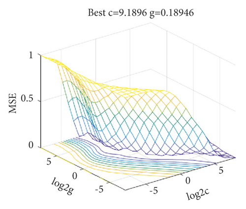
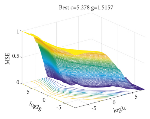
Initially, GS is used for the selection of hyperparameters in the SVR. For the GS-SVR model, C and g are searched in an exponential grid of [2⁻⁸, 2⁸] with step 2^0.1. The evolution of the parameters is shown in Figure 5. The model is trained using 10-fold cross-validation.

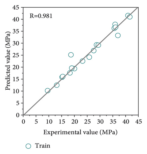
To highlight the superiority of the proposed method in this study, the original SVR model and GS-SVR model were performed on the same training and test set. The model results are shown in Figure 6. It can be clearly observed that compared with the SVR model, the GS-SVR model results have a closer distribution of data points along the diagonal, indicating that the predicted values match better with the experimental values, and the correlation coefficient R exceeds 0.98 for both the training and test sets.

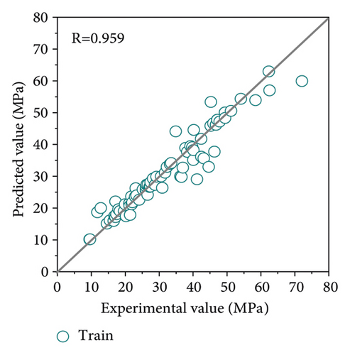
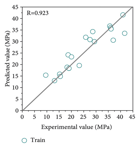
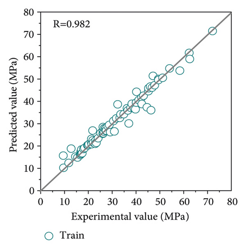
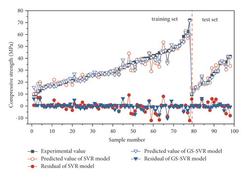
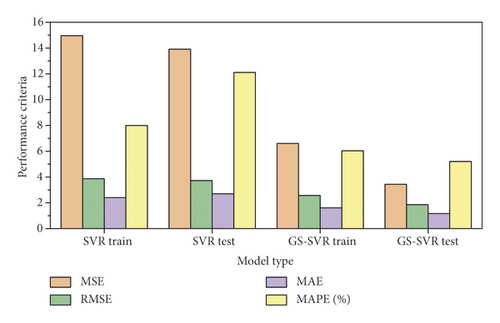
For comparison and evaluation purposes, Figure 7 shows the predicted and experimental values for the training and test sets in more detail. At each sample point, the predicted values agree well with the experimental values, demonstrating the accuracy and effectiveness of the GS-SVR model in capturing the complex nonlinear relationships between the seven input variables and the compressive strength. The error metrics for model training and test are shown in Figure 8. It can be clearly observed from both sets that the four error indicators of the GS-SVR model are smaller, further validating the accuracy and generalization capability of the proposed GS-SVR model.

5. Sensitivity Analysis

The model results in Section 4 show that the compressive strength depends on the input vector consisting of six ingredients and age. However, these variables have almost no deterministic values in a stochastic environment. This uncertainty may cause the deviation of the predicted and actual values of the concrete compressive strength. Therefore, this section focuses on the effect of the random variation degree of each input variable on the compressive strength. According to the statistical characteristics of the dataset given in Table 1, a set of input vectors with deterministic configurations is given in Table 2. The input variables are assumed to be at three different values of degree of stochasticity S₀ = (0.05, 0.1, 0.15). In each stochastic setting, 10⁴ samples were generated using MATLAB. To quantify and compare the degree of influence on the output variable, the sensitivity of the random input to the compressive strength is defined as follows [35, 36].

(7)

where σ and μ are the standard deviation and mean values of the compressive strength, respectively. The distribution of compressive strength for the three randomness settings is shown in Figure 9.

2. Deterministic values of configuration parameters.

Variable	Unit	Value
Cement	kg/m³	230
Fly ash	kg/m³	125
Water	kg/m³	180
Superplasticizer	kg/m³	6
Coarse aggregate	kg/m³	1000
Fine aggregate	kg/m³	800
Age	d	28

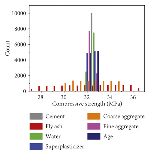
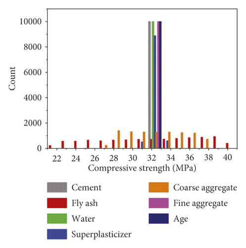
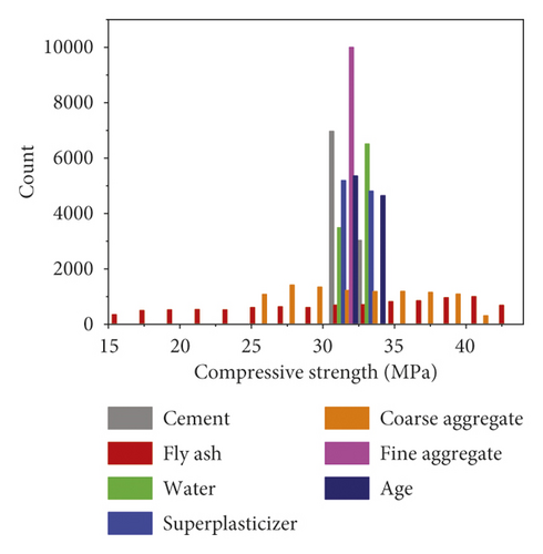
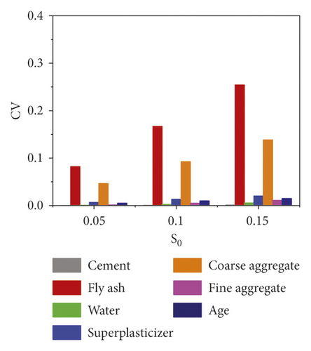
As the randomness S₀ increases, the sensitivity of compressive strength for the three cases is higher. Additionally, among the seven variables, fly ash and coarse aggregate resulted in a more discrete distribution of predicted compressive strength values, where fly ash has the greatest influence on the predicted uncertainty of compressive strength values. This insight might also be observed in Figure 9(d). Designers should take more attention to the design of mix design and compressive strength prediction of concrete with fly ash admixture in stochastic environments.

6. GS-SVR Model-Based Interactive Graphical User Interface

Nowadays, structural designers and engineers prefer to develop more robust and user-friendly software to gain wider applicability. In fact, to ensure that the model developed in this study is useful and practical and for ease of use, a graphical user interface (GUI) was compiled using MATLAB as shown in Figure 10. The whole interface is divided into two main parts: the optimization of hyperparameters and the prediction of output results with known input parameters. The operation of the GUI can be obtained by clicking on the Help menu, and the whole process consists of four main steps.

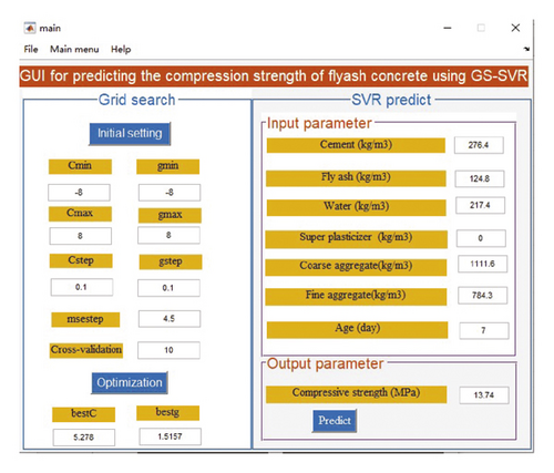
Step 1. Click the Initialize setting button to get the default values of the parameters; these values can also be modified manually.

Step 2. Click the Optimization button to obtain the optimal values of parameters C and g

Step 3. Manually enter each input parameter

Step 4. Click the Predict button to get the final output value

Finally, the compressive strength of fly ash concrete is displayed directly by clicking the Predict button. This GUI was developed mainly for the dataset used in this study, and future optimization of the user interface such as adding new datasets and other influencing parameters can be considered to make the model predictions more accurate.

7. Conclusions

In this work, a hybrid machine learning model GS-SVR was employed to predict the compressive strength of concrete with fly ash admixture and quantity the sensitivity of the compressive strength in the stochastic environment. The main findings are as follows.

(1)
The proposed GS-SVR model can accurately capture the complex nonlinear relationship between the seven input parameters and the compressive strength of concrete with an accuracy R of over 98% in both the training and test phases
(2)
From the performance criteria, the prediction performance of the proposed model is better than that of the original SVR model, which is a promising candidate for evaluating the compressive strength of fly ash concrete
(3)
In the stochastic environment, for the dataset used in this study, the compressive strength of concrete with fly ash admixture is most sensitive to fly ash, followed by the coarse aggregate, and the sensitivity to the other five input variables is weak.
(4)
As the randomness of variables increases, the distribution range of compressive strength becomes wider and the dispersion becomes larger, and designers and engineers should pay more attention to the effect of random variation of fly ash and coarse aggregate on strength uncertainty.
(5)
This study provides a new GUI that can be easily used to predict the compressive strength of fly ash concrete. This tool has been proven to be very successful, exhibiting very reliable predictions. Otherwise, it is idealistic to have some initial estimates of the outcomes before performing any extensive laboratory work or fieldwork.

This work also exhibits several limitations that need to be investigated in the future. First, the dataset used in this study is not large enough, and the effects of aggregate size and water reducing agent type on model prediction accuracy are not studied due to the lack of the dataset. Second, other machine learning algorithms or hybrid models can also be developed appropriately if higher prediction accuracy can be obtained. Finally, the current GUI is relatively simple and rough. As new datasets are added, the model needs to be retrained, and the GUI needs to be further updated and improved.

Conflicts of Interest

The authors declare that they have no conflicts of interest.

Acknowledgments

The authors are grateful for the financial support from the Key Scientific and Technological Research Projects of Henan Province (222102210306).

Open Research

Data Availability

The dataset used to support the findings of this study and the GUI are available from the corresponding author upon request.

References

1 Barbhuiya S., Effects of fly ash and dolomite powder on the properties of self-compacting concrete, Construction and Building Materials. (2011) 25, no. 8, 3301–3305, https://doi.org/10.1016/j.conbuildmat.2011.03.018, 2-s2.0-79955605058.
10.1016/j.conbuildmat.2011.03.018
Web of Science® Google Scholar
2 Fuzail Hashmi A., Shariq M., and Baqi A., Flexural performance of high volume fly ash reinforced concrete beams and slabs, Structures. (2020) 25, 868–880, https://doi.org/10.1016/j.istruc.2020.03.071.
10.1016/j.istruc.2020.03.071
Web of Science® Google Scholar
3 Ahmad W., Ahmad A., Ostrowski K. A., Aslam F., and Joyklad P., A scientometric review of waste material utilization in concrete for sustainable construction, Case Studies in Construction Materials. (2021) 15, https://doi.org/10.1016/j.cscm.2021.e00683.
10.1016/j.cscm.2021.e00683
Google Scholar
4 Ahmad W., Ahmad A., Ostrowski K. A., Aslam F., Joyklad P., and Zajdel P., Sustainable approach of using sugarcane bagasse ash in cement-based composites: a systematic review, Case Studies in Construction Materials. (2021) 15, https://doi.org/10.1016/j.cscm.2021.e00698.
10.1016/j.cscm.2021.e00698
Web of Science® Google Scholar
5 Hefni Y., Zaher Y. A. E., and Wahab M. A., Influence of activation of fly ash on the mechanical properties of concrete, Construction and Building Materials. (2018) 172, 728–734, https://doi.org/10.1016/j.conbuildmat.2018.04.021, 2-s2.0-85056244974.
10.1016/j.conbuildmat.2018.04.021
CAS Web of Science® Google Scholar
6 Hay R. and Ostertag C. P., New insights into the role of fly ash in mitigating alkali-silica reaction (ASR) in concrete, Cement and Concrete Research. (2021) 144.
10.1016/j.cemconres.2021.106440
Google Scholar
7 Kang S., Lloyd Z., Kim T., and Ley M. T., Predicting the compressive strength of fly ash concrete with the Particle model, Cement and Concrete Research. (2020) 137.
10.1016/j.cemconres.2020.106218
Google Scholar
8 Sahmaran M. and Li V. C., Durability properties of micro-cracked ECC containing high volumes fly ash, Cement and Concrete Research. (2009) 39, no. 11, 1033–1043.
10.1016/j.cemconres.2009.07.009
CAS Web of Science® Google Scholar
9 Chopra P., Sharma R. K., Kumar M., and Chopra T., Comparison of machine learning techniques for the prediction of compressive strength of concrete, Advances in Civil Engineering. (2018) 2018, 9, 5481705, https://doi.org/10.1155/2018/5481705, 2-s2.0-85046026842.
10.1155/2018/5481705
Web of Science® Google Scholar
10 Chou J.-S. and Pham A.-D., Enhanced artificial intelligence for ensemble approach to predicting high performance concrete compressive strength, Construction and Building Materials. (2013) 49, 554–563, https://doi.org/10.1016/j.conbuildmat.2013.08.078, 2-s2.0-84884786542.
10.1016/j.conbuildmat.2013.08.078
Web of Science® Google Scholar
11 Farooq F., Akbar A., Khushnood R. A., Muhammad W. L. B., Rehman S. K. U., and Javed M. F., Experimental investigation of hybrid carbon nanotubes and graphite nanoplatelets on rheology, shrinkage, mechanical, and microstructure of SCCM, Materials. (2020) 13, no. 1, https://doi.org/10.3390/ma13010230.
10.3390/ma13010230
Web of Science® Google Scholar
12 Deifalla A. F., Zapris A. G., and Chalioris C. E., Multivariable regression strength model for steel fiber-reinforced concrete beams under torsion, Materials. (2021) 14, no. 14, https://doi.org/10.3390/ma14143889.
10.3390/ma14143889
PubMed Google Scholar
13 Sucharda O., Pajak M., Ponikiewski T., and Konecny P., Identification of mechanical and fracture properties of self-compacting concrete beams with different types of steel fibres using inverse analysis, Construction and Building Materials. (2017) 138, 263–275, https://doi.org/10.1016/j.conbuildmat.2017.01.077, 2-s2.0-85012243994.
10.1016/j.conbuildmat.2017.01.077
CAS Web of Science® Google Scholar
14 Azimi-Pour M., Eskandari-Naddaf H., and Pakzad A., Linear and non-linear SVM prediction for fresh properties and compressive strength of high volume fly ash self-compacting concrete, Construction and Building Materials. (2020) 230, https://doi.org/10.1016/j.conbuildmat.2019.117021.
10.1016/j.conbuildmat.2019.117021
Web of Science® Google Scholar
15 Zhang J., Ma G., Huang Y., Sun J., Aslani F., and Nener B., Modelling uniaxial compressive strength of lightweight self-compacting concrete using random forest regression, Construction and Building Materials. (2019) 210, 713–719, https://doi.org/10.1016/j.conbuildmat.2019.03.189, 2-s2.0-85063604391.
10.1016/j.conbuildmat.2019.03.189
Web of Science® Google Scholar
16 Golafshani E. M. and Ashour A., Prediction of self-compacting concrete elastic modulus using two symbolic regression techniques, Automation in Construction. (2016) 64, 7–19, https://doi.org/10.1016/j.autcon.2015.12.026, 2-s2.0-84958231069.
10.1016/j.autcon.2015.12.026
Web of Science® Google Scholar
17 Saha P., Debnath P., and Thomas P., Prediction of fresh and hardened properties of self-compacting concrete using support vector regression approach, Neural Computing & Applications. (2020) 32, no. 12, 7995–8010, https://doi.org/10.1007/s00521-019-04267-w, 2-s2.0-85067820396.
10.1007/s00521-019-04267-w
Web of Science® Google Scholar
18 Neira P., Bennun L., Pradena M., and Gomez J., Prediction of concrete compressive strength through artificial neural networks, Građevinar. (2020) 72, no. 7, 585–592.
Google Scholar
19 Kostic S. and Vasovic D., Prediction model for compressive strength of basic concrete mixture using artificial neural networks, Neural Computing & Applications. (2015) 26, no. 5, 1005–1024.
10.1007/s00521-014-1763-1
Web of Science® Google Scholar
20 Duan Z. H., Kou S. C., and Poon C. S., Prediction of compressive strength of recycled aggregate concrete using artificial neural networks, Construction and Building Materials. (2013) 40, 1200–1206, https://doi.org/10.1016/j.conbuildmat.2012.04.063, 2-s2.0-85027952094.
10.1016/j.conbuildmat.2012.04.063
Web of Science® Google Scholar
21 Parthiban P. and Karthikeyan J., Artificial neural network to predict the compressive strength of semilightweight concrete containing ultrafine GGBS, Journal of Testing and Evaluation. (2019) 48, no. 2, 795–810, https://doi.org/10.1520/jte20180597.
10.1520/JTE20180597
Google Scholar
22 Zhang J., Xu J., Liu C., and Zheng J., Prediction of rubber fiber concrete strength using extreme learning machine, Frontiers in Materials. (2021) 7, no. 465, https://doi.org/10.3389/fmats.2020.582635.
10.3389/fmats.2020.582635
PubMed Google Scholar
23 Wang Y. R., Lu Y. L., and Chiang D. L., Adapting artificial intelligence to improve in situ concrete compressive strength estimations in rebound hammer tests, Frontiers in Materials. (2020) 7, no. 365, https://doi.org/10.3389/fmats.2020.568870.
10.3389/fmats.2020.568870
Google Scholar
24 Ly H. B., Nguyen T. A., Mai H. V. T., and Tran V. Q., Development of deep neural network model to predict the compressive strength of rubber concrete, Construction and Building Materials. (2021) 301, https://doi.org/10.1016/j.conbuildmat.2021.124081.
10.1016/j.conbuildmat.2021.124081
Google Scholar
25 Han Q., Gui C., Xu J., and Lacidogna G., A generalized method to predict the compressive strength of high-performance concrete by improved random forest algorithm, Construction and Building Materials. (2019) 226, 734–742, https://doi.org/10.1016/j.conbuildmat.2019.07.315, 2-s2.0-85073654077.
10.1016/j.conbuildmat.2019.07.315
Web of Science® Google Scholar
26 Farooq F., Czarnecki S., Niewiadomski P., Aslam F., Alabduljabbar H., Ostrowski K. A., Sliwa-Wieczorek K., Nowobilski T., and Malazdrewicz S., A comparative study for the prediction of the compressive strength of self-compacting concrete modified with fly ash, Materials. (2021) 14, no. 17, https://doi.org/10.3390/ma14174934.
10.3390/ma14174934
Web of Science® Google Scholar
27 Zhang X., Akber M. Z., and Zheng W., Prediction of seven-day compressive strength of field concrete, Construction and Building Materials. (2021) 305, 124604, https://doi.org/10.1016/j.conbuildmat.2021.124604.
10.1016/j.conbuildmat.2021.124604
Web of Science® Google Scholar
28 Nguyen K. T., Nguyen Q. D., Le T. A., Shin J., and Lee K., Analyzing the compressive strength of green fly ash based geopolymer concrete using experiment and machine learning approaches, Construction and Building Materials. (2020) 247, 118581, https://doi.org/10.1016/j.conbuildmat.2020.118581.
10.1016/j.conbuildmat.2020.118581
CAS Web of Science® Google Scholar
29 Al-Shamiri A. K., Kim J. H., Yuan T.-F., and Yoon Y. S., Modeling the compressive strength of high-strength concrete: an extreme learning approach, Construction and Building Materials. (2019) 208, 204–219, https://doi.org/10.1016/j.conbuildmat.2019.02.165, 2-s2.0-85062350517.
10.1016/j.conbuildmat.2019.02.165
Web of Science® Google Scholar
30 Jiang W., Xie Y. J., Li W. X., Wu J. X., and Long G. C., Prediction of the splitting tensile strength of the bonding interface by combining the support vector machine with the particle swarm optimization algorithm, Engineering Structures. (2021) 230.
10.1016/j.engstruct.2020.111696
Google Scholar
31 Chang C.-C. and Lin C.-J., Training v-support vector regression: theory and algorithms, Neural Computation. (2002) 14, no. 8, 1959–1977, https://doi.org/10.1162/089976602760128081, 2-s2.0-0038895405.
10.1162/089976602760128081
PubMed Web of Science® Google Scholar
32 Chang C.-C. and Lin C.-J., LIBSVM: a library for support vector machines, ACM Transactions on Intelligent Systems and Technology. (2011) 2, no. 3, 27, https://doi.org/10.1145/1961189.1961199, 2-s2.0-79955702502.
10.1145/1961189.1961199
PubMed Web of Science® Google Scholar
33 Liu Y. R., Wang L., and Gu K. X., A support vector regression (SVR)-based method for dynamic load identification using heterogeneous responses under interval uncertainties, Applied Soft Computing. (2021) 110, https://doi.org/10.1016/j.asoc.2021.107599.
10.1016/j.asoc.2021.107599
Google Scholar
34 Hadzima-Nyarko M., Nyarko E. K., Ademovic N., Milicevic I., and Sipos T. K., Modelling the influence of waste rubber on compressive strength of concrete by artificial neural networks, Materials. (2019) 12, no. 4, https://doi.org/10.3390/ma12040561, 2-s2.0-85061537005.
10.3390/ma12040561
PubMed Google Scholar
35 Nguyen M. S. T., Trinh M. C., and Kim S. E., Uncertainty quantification of ultimate compressive strength of CCFST columns using hybrid machine learning model, Engineering with Computers. (2021) https://doi.org/10.1007/s00366-021-01339-1.
10.1007/s00366-021-01339-1
Google Scholar
36 Nguyen M. S. T. and Kim S. E., A hybrid machine learning approach in prediction and uncertainty quantification of ultimate compressive strength of RCFST columns, Construction and Building Materials. (2021) 302, https://doi.org/10.1016/j.conbuildmat.2021.124208.
10.1016/j.conbuildmat.2021.124208
Google Scholar

Citing Literature

All articles

Hybridizing Grid Search and Support Vector Regression to Predict the Compressive Strength of Fly Ash Concrete

Abstract

1. Introduction