Volume 2022, Issue 1 2659826

Research Article

Open Access

Energy Source Allocation Decision-Making in Textile Industry: A Novel Symmetric and Asymmetric Spherical Fuzzy Linear Optimization Approach

Sajida Kousar,

Sajida Kousar

orcid.org/0000-0001-8157-7909

Department of Mathematics and Statistics, International Islamic University Islamabad, Pakistan iiu.edu.pk

Search for more papers by this author

Urooj Shafqat,

Urooj Shafqat

orcid.org/0000-0003-3246-7281

Department of Mathematics and Statistics, International Islamic University Islamabad, Pakistan iiu.edu.pk

Search for more papers by this author

Nasreen Kausar,

Nasreen Kausar

orcid.org/0000-0002-8659-0747

Department of Mathematics, Faculty of Arts and Sciences, Yildiz Technical University, Esenler, 34210, Istanbul, Turkey yildiz.edu.tr

Search for more papers by this author

Dragan Pamucar,

Dragan Pamucar

orcid.org/0000-0001-8522-1942

Department of Logistics, University of Defence in Belgrade, Belgrade, Serbia uo.mod.gov.rs

Search for more papers by this author

Yaé Ulrich Gaba,

Corresponding Author

Yaé Ulrich Gaba

[email protected]

orcid.org/0000-0001-8128-9704

Quantum Leap Africa (QLA), AIMS Rwanda Center, Remera Sector KN 3, Kigali, Rwanda

Institut de Mathématiques et de Sciences Physiques (IMSP/UAC), Laboratoire de Topologie Fondamentale, Computationnelle et leurs Applications (Lab-ToFoCApp), BP 613, Porto-Novo, Benin imsp-benin.com

African Center for Advanced Studies, P.O. Box 4477, Yaounde, Cameroon

Search for more papers by this author

Sajida Kousar,

Sajida Kousar

orcid.org/0000-0001-8157-7909

Department of Mathematics and Statistics, International Islamic University Islamabad, Pakistan iiu.edu.pk

Search for more papers by this author

Urooj Shafqat,

Urooj Shafqat

orcid.org/0000-0003-3246-7281

Department of Mathematics and Statistics, International Islamic University Islamabad, Pakistan iiu.edu.pk

Search for more papers by this author

Nasreen Kausar,

Nasreen Kausar

orcid.org/0000-0002-8659-0747

Department of Mathematics, Faculty of Arts and Sciences, Yildiz Technical University, Esenler, 34210, Istanbul, Turkey yildiz.edu.tr

Search for more papers by this author

Dragan Pamucar,

Dragan Pamucar

orcid.org/0000-0001-8522-1942

Department of Logistics, University of Defence in Belgrade, Belgrade, Serbia uo.mod.gov.rs

Search for more papers by this author

Yaé Ulrich Gaba,

Corresponding Author

Yaé Ulrich Gaba

[email protected]

orcid.org/0000-0001-8128-9704

Quantum Leap Africa (QLA), AIMS Rwanda Center, Remera Sector KN 3, Kigali, Rwanda

Institut de Mathématiques et de Sciences Physiques (IMSP/UAC), Laboratoire de Topologie Fondamentale, Computationnelle et leurs Applications (Lab-ToFoCApp), BP 613, Porto-Novo, Benin imsp-benin.com

African Center for Advanced Studies, P.O. Box 4477, Yaounde, Cameroon

Search for more papers by this author

First published: 16 February 2022

https://doi.org/10.1155/2022/2659826

Citations: 2

Academic Editor: Akif Akgul

Share a link

Email
Wechat
Bluesky

Abstract

In this study, the authors extended the concept of spherical fuzzy optimization models by considering different parameters of spherical fuzzy linear programming problem as symmetric and asymmetric spherical numbers. Eight spherical fuzzy linear programming models are discussed by converting decision variables, parameters, and coefficients of objective function and constraints into symmetric and asymmetric spherical fuzzy numbers. To verify the validity and efficiency of this study in contrast with a linear programming numerical and a physical energy optimization model for the textile industry is considered. The application of these symmetric and asymmetric spherical fuzzy optimization models is discussed along with the postoptimal analysis of the best optimization models that provide the feasible and most optimal solution.

1. Introduction

Growing urbanization is directly related to the increase in energy demands, usage, and cost. Energy optimization is globally targeted by every sector. Mostly, an industrial sector is the one who consumed most of the produced or natural energy. The key factor of rising production cost in the industrial sector is abrupt energy usage. Since industrial sectors cannot ignore this factor, getting help through mathematical modeling such as optimizing cost, profits, loss, and energy for such matters is sane act. A lot of work is performed for the optimal utilization of energy in different areas as Wang et al. presented their general guidelines regarding energy optimization in iron and steel industry by using mass-thermal network optimization [1]. Ullah et al. presented bio-inspired energy optimization techniques with the purpose of power scheduling in an office [2]. According to Ozturk et al., energy consumption could be decreased by using the waste-heat recovery systems for the industrial sector so they presented eighty-five techniques for the reduction of energy consumption in their study where thirteen of them were prioritized and applied as energy-efficient techniques [3]. Kimutai [4] proposed the physical energy optimization model for the textile industry and optimized the energy cost by using linear programming (LP). In the manufacturing sector, textile industries are considered major energy consumption units globally due to their several production stages. In the textile industry, mostly electricity and fuel, such as charcoal and petroleum, are used to create all the required kinds of energy. In Pakistan, this particular industrial sector is having a great share up to 8.5% towards GDP (gross domestic product) and considered Asia’s 8th largest textile exporter [5]. Pakistan is having a huge textile industrial sector and now facing many uncertainties due to the unpredicted policy shift 2020–25 and COVID. According to National Electric Power Regulatory Authority’s (NEPRA) report, one energy unit fluctuation cost causes almost 4 to 5 hours closure in the production of textile’s products [6]. To overcome this loss, it is best to optimize the usage and wastage of energy as much as possible. The most extensively adopted procedure for the optimal solution of modeled problem was linear programming (LP) due to its easy applicable nature that was first introduced by Kantorovich [7]. Advancement in this traditional LP generated several extensions such as bi-level LP, multilevel LP, and multiobjective. These LP extensions are highly applicable in real life such as it gave optimized solutions for transportation, supply chain, energy, profit, loss, and cost optimization problems.

Huge modification happened in linear programming after the introduction of fuzzy sets by Zadeh [8]. Fuzzy linear programming was introduced by Zimmerman [9], who originated the technique to solve the multiobjective linear programming in a fuzzy environment. This method was defined according to the natural environmental uncertainties as all the optimization conditions can be considered in fuzzy. Improvements are continuously occurring till now; firstly, membership degree was considered well enough to understand decision-makers choices, but Atanssove [10] created an intuitionistic fuzzy set dealing with the degree of membership and nonmembership clearly, recognizing the choice of an element from the decision set. This definition of the intuitionistic fuzzy set became another reason for improvement in optimization techniques, and firstly, intuitionistic fuzzy (IF) optimization got revealed by Angelov [11]. A lot of work has been carried out in intuitionistic fuzzy linear programming (IFLP). Afterwards, Yager presented the concept of another generalization of fuzzy sets and named it Pythagorean fuzzy set by refining the condition that membership and nonmembership can be independent of each other and their sum of squares must be less than 1 [12]. In 1999, Smarandache [13] introduced a neutrosophic set, which covers the third predictable choice of decision-makers that might be neutral or indeterminacy. In the neutrosophic environment, many optimization models were considered and solved by Ahmad et al. [14, 15].

Recently, a spherical fuzzy set has been introduced by Gundogdu and Kahraman [16]. A spherical fuzzy set is defined with the compliance of positive, neutral, and negative membership functions under the condition that the sum of their squares must be less than 1 providing more general way to cope with uncertainty. It is considered that a spherical fuzzy set is a superset of fuzzy, Pythagorean fuzzy, and intuitionistic fuzzy sets. Ahmad and Adhami [17] presented their work on spherical fuzzy linear programming problem (SFLPP). They presented different types of optimization models under the spherical fuzzy (SF) environment. In this study, we are presenting symmetric and asymmetric energy optimization models inspired by the work of Ahmad and Adhami [17]. For this purpose, the LP model for the textile industry is considered in the spherical fuzzy environment as a numeric example to validate the working of generated energy optimization models in the SF environment. For the conversion of LP into SFLP, parameters were considered spherical fuzzy numbers (SFNs). By targeting each parameter one by one, different SF optimization models are constructed. Every model further contains two submodels in it on the basis of symmetric spherical fuzzy number (SSFN) and asymmetric spherical fuzzy numbers (ASFN) parameters. The deterministic version corresponding to SFNs is based on the spherical fuzzy set theory. Conclusions are based on the application of these spherical fuzzy models on the energy optimization model. The postoptimal analysis of the best feasible optimized SF model is also discussed.

2. Preliminaries

A spherical fuzzy set (SFS) is defined by Rafiq et al. [18] as the following set:

(1)

Considering U the universal discourse and

representing spherical fuzzy set such that

(2)

where

is positive membership degree, and

and

is representing neutral and negative membership degree of each u ∈ U, respectively, to

. A spherical fuzzy number is a fuzzy number

with positive, neutral, and negative membership functions defined as

(3)

Here, α, β, γ ∈ [0,1] such that 0 ≤ α² + β² + γ² ≤ 1. Let

and

are two spherical fuzzy numbers, and then, the algebraic operations [18] between them are defined as follows:

A SFN will be considered symmetric spherical fuzzy number (SSFN) if there exists a relation between positive and neutral, positive, and negative membership. For example,

(4)

where λ > 0, k > 1, and λ, k ∈ ℝ; otherwise, it is considered asymmetric spherical fuzzy number (ASFN).

3. Spherical Fuzzy Linear Programming Problem

Ideally for optimal solution of mathematically modeled problem, linear programming (LP) is considered the most convenient way [7]. Since this LP does not accommodate the fuzziness of nature, the best real-life modeled problem solution requires a method of fuzzy optimization. A lot of work is already carried out for fuzzy optimization modeling by utilizing different techniques such as intuitionistic fuzzy linear programming [11, 12] and neutrosophic LP [14–19]. Ahmad and Adhami presented different models for the solution of spherical fuzzy LP [17]. By continuing their idea for SF modeling, different spherical fuzzy models are constructed in this study. In the first model, only constraint coefficients were considered spherical fuzzy numbers, whereas all the other decision variables and parameters are real quantities. In the second model, two factors demand and constraint coefficients are taken as SFNs, while cost is taken as a real number. In the third model, other than decision variables, all the other factors are considered in the spherical fuzzy number, whereas in the fourth model, the cost and demand are in SF numbers. Table 1 is designed to illustrate all these cases.

Table 1. Spherical fuzzy linear programming models.

Model	Symmetric spherical fuzzy model (a)	Asymmetric spherical fuzzy model (b)
I	subjected to	subjected to

II	subjected to , ∀j = 1,2,3 … l	subjected to

III	subjected to	subjected to

IV	subjected to , ∀j = 1,2,3 … l	subjected to , ∀j = 1,2,3 … l

In Table 1, , , and are symmetric spherical fuzzy, , , and asymmetric spherical fuzzy parameters, and s, d, c real-valued parameters.

4. Numerical Example

Consider the following linear programming problem:

(5)

(6)

(7)

The SSF and ASF for the above LP are presented in Table 2.

Table 2. Spherical fuzzy linear programming models.

Model	Symmetric spherical fuzzy model (a)	Asymmetric spherical fuzzy model (b)
I	Max Z = 5x + 3y subjected to ,	Max Z = 5x + 3y subjected to
II	Max Z = 5x + 3y subjected to ,	Max Z = 5x + 3y subjected to
III	subjected to ,	subjected to
IV	subjected to ,	subjected to

In Table 2, , , , , , and , , , , . Since objective function is needed to be maximize, preference will be given to the model with a higher optimal value. By solving 0.3 in different fuzzy and crisp environment as in fuzzy, intuitionistic fuzzy, and spherical fuzzy, we obtain the results shown in Table 3).

Table 3. Comparison of LP and different fuzzy optimization models for the numerical example.

Optimization model	Objective function	x	y
LP	12.3684	1.05263	2.36842
FLP	15.13159	1.44737	2.63158
IFLP	16.31579	1.052632	2.368421
SSF Model-I	22.1171	3.119093	2.173913
ASF Model-I	16.58654	1.442308	3.125
SSF Model-II	12.97593	1.100301	2.491472
ASF Model-II	12.71875	1.0625	2.46875
SSF Model-III	9.691474	1.100301	2.491472
ASF Model-III	8.957813	1.0625	2.46875
SSF Model-IV	6.808947	0.684211	1.8894744
ASF Model-IV	6.660789	0.768421	1.878947

From Table 3, it is clear that SSF model-I results in the highest optimal solution value. Since the solution of LP is 12.3684 and we are looking for more better feasible solution, all those models whose values are greater; that is, higher than LP output is considered better. Here, in Table 3, we obtain that

(8)

where the remaining models result in a value less than LP solution so these are not considered better than LP. All the models are providing feasible solution, and the best one is provided by SSF model-I as it results in the highest objective output.

5. Application

To elaborate the working efficiency of the above-defined SSF and ASF optimization models of our study, we construct an energy optimization model for the textile industry with five stages shown in Figure 1.

Details are in the caption following the image — **Figure 1**
Open in figure viewer PowerPoint

Production stages.

Suppose X_i is the number of units of product that processed at stage i. In the objective function, the cost coefficients are according to the type of energy used for the preparation of per unit product of stage i. D_i is the monthly demand of each product X_i and availability of working hours that helped to form the following demand constraint equations according to the stages presented in Figure 1:

(9)

Each stage in Figure 1 is also presenting the production cost per unit of each stage’s product along with information about how much quantity is going to be processed further in the next stage by considering electricity cost 20.62 PKR/kWh, fuel (furnace oil) price PKR85.68/litre, and LPG cost at the rate of PKR19.4103/litre [20, 21]. The last constraint is regarding availability of total working time and production rate, that is, how much hours are needed for the production of 1 kg product of spinning, weaving, and final stages. Objective function constructed through Figure 1 is

(10)

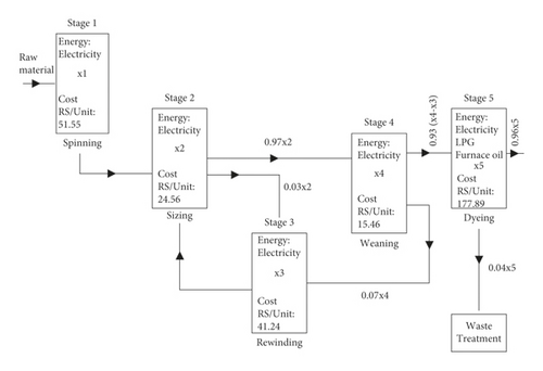
To conduct optimization in the spherical fuzzy environment, the uncertainty in demand, supply parameters, and energy cost per unit fluctuation is kept in mind and considered symmetric and asymmetric SFNs. The considered positive, neutral, and negative membership degree of acceptance is throughout (0.5, 0.3, 0.2).

6. Model-I(a)

subjected to , ∀j = 1,2, …, 5, where spherical fuzzy coefficients are considered symmetric with x_i real decision variables where d_j is real-valued demands. After the conversion of an inconsideration energy optimization model for the textile industry into the symmetric spherical fuzzy model-I(a), it is represented as follows:

Cost set is C = {c_i, i = 1,2,3,4,5} C = {51.55, 24.5653, 41.24, 15.46, 177.8921}, where symmetric spherical fuzzy constraint coefficients are

(11)

with the monthly production demand in kg for three products and total availability of working hours in a month as D = {d₁ = 400, d₂ = 600, d₃ = 20000, d₄ = 720}. Mathematically, symmetric spherical fuzzy energy optimization is framed as follows:

(12)

Subjected to

(13)

The above symmetric spherical fuzzy liner programming model is then converted into LP, and the following defuzzified constraints are obtained:

(14)

7. Model-I(b)

Now in this model, the spherical fuzzy coefficients are considered asymmetric with x_i real-valued decision variables with d_j, c_i, which are real demands and costs.

For this purpose, by changing the values of spherical fuzzy coefficients by asymmetric spherical fuzzy in the above model-I(a) in (9) for the textile industry, the following changes occurred:

(15)

The monthly production demand in kg for three products and total availability of working hours in a month are D = {d₁ = 400, d₂ = 600, d₃ = 20000, d₄ = 720}. The asymmetric spherical fuzzy energy optimization model is

(16)

subjected to constraints

(17)

The defuzzyfied form of the above ASF linear programming model is given as

(18)

8. Model-II(a)

In this model, constraint coefficients and demand is considered in the symmetric spherical fuzzy number and cost remains unchanged as follows:

(19)

The symmetric SF energy optimization model-II(a) for the textile industry becomes

(20)

Under the constraints

(21)

converting the above constraint into LP:

(22)

Solve the objective function 0.13 subjected to set of constraints 0.15 to obtain the solution.

9. Model-II(b)

In this model, constraint coefficients and demand is considered asymmetric spherical fuzzy number:

(23)

The asymmetric SF energy optimization model-II(b) with objective function 0.13 for the textile industry under the constraints:

(24)

converting the above constraint into real-valued:

(25)

10. Model-III(a)

In this model, all the cost and demand coefficients are in SSFNs, so here the objective function is expressed as follows:

(26)

under the constraints

(27)

after converting the above model into general LP, 0.15 becomes required constraints for the objective function:

(28)

11. Model-III(b)

By solving objective function,

(29)

Under the subjected constraint 0.16, we obtain an infeasible solution after converting into LP objective function by using the weight formula,

12. Model-IV(a)

In this model, we considered cost and demand (right-hand side of constraint equations) a symmetric spherical fuzzy number. The spherical fuzzy energy optimization model for the textile industry according to this model is as follows:

(30)

subjected to

(31)

converting the above model into LP, we obtain

(32)

under the real constraints

(33)

13. Model-IV(b)

(34)

Subjected to

(35)

subjected to

(36)

converting the above model into LP, we obtain

(37)

under defuzzified constraints

(38)

Table 4 shows the optimal output we obtained through different models.

14. Postoptimal Analysis

In present study eight models with different symmetric and asymmetric spherical fuzzy changes were tried. Out of eight models only five models provided us a feasible solution for spherical fuzzy energy optimization model 0.5 and one of them provided the best optimal result as compared to all SF models and LP as shown in Table 4 while all the other spherical fuzzy models resulted those objective values, which are much higher than real LP. Overall, if we combine the objective value in the form of inequality keeping LP greatest we get:

(39)

the objective values obtained from these methods also satisfy the relation as

(40)

Table 4. Optimal solutions.

Optimization model	Objective value	x₁	x₂	x₃	x₄	x₅
LP	5987499	24195.38	23759.38	2326.043	23046.59	20833.33
IFLP	5927615.1	24159.4	23759.4	874.104	23046.6	20833.33
Model-I(a)	5702683	21744.58	21344.58	3639.78	21451.3	20100.50
Model-I(b)	Infeasible solution	0	0	0	0	0
Model-II(a)	5717777.8	21851.93	21416.93	3652.12	21524.02	20135.68
Model-II(b)	Infeasible solution	0	0	0	0	0
Model-III(a)	6027917.33	21851.93	21416.93	3652.12	21524.02	20135.68
Model-III(b)	Infeasible solution	0	0	0	0	0
Model-IV(a)	6333697.02	24273.59	23838.59	2333.8	23123.43	20869.79
Model-IV(b)	6448227.44	24280.77	23843.57	2334.28	23128.26	20872.08

Except one ASF model, all the other ASF (models-I, II, III) energy optimization models gave “Infeasible solution” in 0.5 and one ASF model-IV, which provided a solution that have the most highest optimal value (greater than LP) where objective function was needed to minimize, whereas in 0.3 where the objective function was needed to maximize the similar models, ASF (models-I, II, III) provided feasible solution, but other than SSF and AS (models- I, II), all the other remaining models provided outputs less than LP; that is, the outputs of these models are much lesser than LP’s outputs. Here, in the following tables, the sensitivity report and limits of all those SF models in 0.5 are discussed whose optimal solutions were not greater than the LP textile energy model.

In Table 5 the flexibility regarding allowable change in optimal and feasible conditions is mentioned. Since solution is effected by both and impacts the efficiency of model, how much cost and demand fluctuation can be handled by these models in 0.5 is discussed, whereas in Tables 6, 7 and 8 the feasibility range of the decision variable is discussed along with the optimal solution between that range. In Table 9 the validity range of all the parameters and decision variables of the best optimal model for 0.5 is mentioned. According to the above postoptimal analysis, we obtain the following information about the range of each factor of the energy optimization model in a spherical environment. SSF model-I(a) is providing a minimal optimal value of the objective function for a longer range of coefficients that insure the feasibility for a huge change in 0.5. In both situations, where objective function is needed to maximize 0.3 or to minimize 0.5, SSF model-I(a) provided the best results.

Table 5. Model-I(a) sensitivity analysis report.

Variables	Final value	Reduced cost	Objective coefficient	Allowable increase	Allowable decrease
x₁	21744.57	0	51.55	1E+30	51.55
x₂	21344.57	0	24.56	1E+30	98.68
x₃	3639.78	0	41.24	1E+30	578.68
x₄	21451.3	0	15.46	1E+30	98.19
x₅	20100.50	0	177.89	1E+30	279.64

Constraint	Final value	Shadow price	RHS	Allowable increase	Allowable decrease

1	400	51.55	400	21923.36	21744.57
2	4.55E–13	–41.24	0	3639.78	1E+30
3	0	78.4	0	1E+30	21451.3
4	600	101.75	600	13462.94	20700.50
5	20000	281.05	20000	9685.38	20000
6	489.80	0	720	1E+30	230.19

Table 6. Model-I(a) limits report.

Variable	Values	Lower limit	Objective result	Upper limit	Objective result
x₁	21744.57	21744.57	5702683.001	43667.94	6832832.271
x₂	21344.57	21344.57	5702683.001	21344.57	5702683.001
x₃	3639.78	3639.78	5702683.001	3639.78	5702683.001
x₄	21451.3	21451.3	5702683.001	21451.30	5702683.001
x₅	20100.50	20100.50	5702683.001	20100.50	5702683.001

Table 7. Model-II(a) sensitivity analysis report.

Variables	Final value	Reduced cost	Objective coefficient	Allowable increase	Allowable decrease
x₁	21851.93	0	51.55	1E+30	51.55
x₂	21416.93	0	24.56	1E+30	98.68
x₃	3652.12	0	41.24	1E+30	578.68
x₄	21524.02	0	15.46	1E+30	98.19
x₅	20135.68	0	177.89	1E+30	279.64

Constraint	Final value	Shadow price	RHS	Allowable increase	Allowable decrease

1	435	51.55	435	25085.47	21851.9
2	4.55E−13	−41.24	0	3652.12	1E+30
3	0	78.4	0	1E+30	21524.02
4	635	101.75	635	15404.76	20770.68
5	20035	281.045	20035	11082.36	20035
6	491.60	0	755	1E+30	263.4

Table 8. Model-II(a) limits report.

Variable	Values	Lower limit	Objective result	Upper limit	Objective result
x₁	21851.93	21851.93	5717777.832	46937.41	7010934.09
x₂	21416.93	21416.93	5717777.832	21416.93	5717777.832
x₃	3652.12	3652.12	5717777.832	3652.12	5717777.832
x₄	21524.02	21524.02	5717777.832	21524.02	5717777.832
x₅	20135.68	20135.68	5717777.832	20135.69	5717777.832

Table 9. Validity range of SSF-I(a).

Factors	SSF model-I(a)	Range
x₁	21744.56 units	21923.38 unit
x₂	21344.56 units	0
x₃	3539.73 units	0
x₄	21451.3 units	0 unit
x₅	20100 units	0 unit
c₁	51.55 Rs./unit	51.55 Rs/unit
c₂	24.56 Rs./units	98.68 Rs/unit
c₃	41.24 Rs./units	578.71 Rs/unit
c₄	15.46 Rs./units	98.2 Rs/unit
c₅	177.89 Rs./units	279.64 Rs/unit
d₁	400 kg/month	43667 kg/month
d₂	0	3639.78 kg/month
d₃	0	21451.3 kg/month
d₄	20000 kg/month	29685.39 kg/month
d₅	600 kg/month	43163.44 kg/month
d₆	720 working hours/month	489.81 hours/month

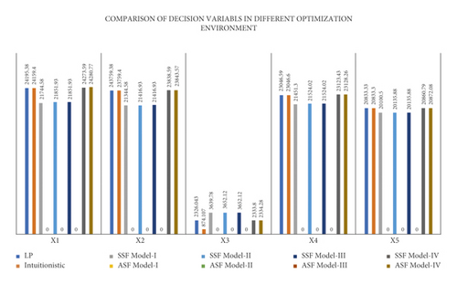
From Figure 2 it is clearly seen that all the decision variables in SSF model-I for 0.5 is having least value as compared to other models except x₃. This x₃ is providing its minimal value in the intuitionistic fuzzy environment.

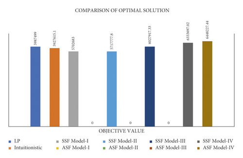
In Figure 3 an objective value of 0.5 in different fuzzy and LP environments is graphically presented. Three bars in the right-hand side denote ASF models and are clearly higher than even LP’s bar. Therefore, they are not considered the best models for 0.5. SSF model-I is providing the best results as compared to others.

15. Conclusion

Spherical fuzzy set (SFS) is a well-known generalization of widely studied fuzzy sets, and significant research has been carried out to investigate SFS set theocratic properties and applications in other fields. Due to the involvement of positive, neutral, and negative grades, SFS can handle uncertainties better than fuzzy sets. In this article, linear optimization is carried out by utilizing spherical fuzzy numbers. The method is superior to previously defined techniques as shown in.

(1)
Due to the spherical region, parameters are highly flexible and can provide optimal solution between a long range
(2)
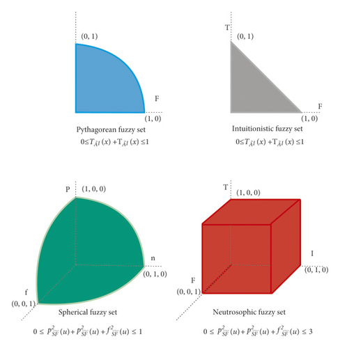
Spherical fuzzy set is a super set of the intuitionistic and Pythagorean fuzzy set, so it will cover more area graphically (see Figure 4) and can easily target those points for solution that are far away to those points, which are obtained through LP or IF technique
(3)
No need to construct or change a model for a huge change due to long-range flexibility of parameters

The method can be used in any decision-making problem simply by identifying the objectives, parameters, and the constraints imposed to maximize or minimize the objective. In recent years, the fuzzy set and its generalizations are used widely in decision-making related to real-life problems [22, 23]. Any advancement in basic fuzzy set theocratic concepts will ultimately improve the accuracy of its implementation by incorporating the imprecision and vagueness in the data. Spherical fuzzy optimization techniques can be used to find the suitable weights for the best criteria over others in the decision-making process. [24–26].

Conflicts of Interest

The authors declare that there are no conflicts of interest regarding the publication of this article.

Authors’ Contributions

All authors contributed equally to the preparation of this manuscript.

Acknowledgments

The fifth author (YUG) would like to acknowledge that this publication was made possible by a grant from the Carnegie Corporation of New York.

Open Research

Data Availability

No data were used to support this study.

References

1 Wang R. Q., Jiang L., Wang Y. D., and Roskilly A. P., Energy saving technologies and mass-thermal network optimization for decarbonized iron and steel industry: a review, Journal of Cleaner Production. (2020) 274, 122997, https://doi.org/10.1016/j.jclepro.2020.122997.
10.1016/j.jclepro.2020.122997
CAS Web of Science® Google Scholar
2 Ullah I., Khitab Z., Khan M., and Hussain S., An efficient energy management in office using bio-inspired energy optimization algorithms, Processes. (2019) 7, no. 3, 142, https://doi.org/10.3390/pr7030142, 2-s2.0-85062916474.
10.3390/pr7030142
Web of Science® Google Scholar
3 Ozturk E., Cinperi N. C., and Kitis M., Improving energy efficiency using the most appropriate techniques in an integrated woolen textile facility, Journal of Cleaner Production. (2020) 254, 120145, https://doi.org/10.1016/j.jclepro.2020.120145.
10.1016/j.jclepro.2020.120145
Web of Science® Google Scholar
4 Kimutai I., Maina P., and Makokha A., Energy optimization model using linear programming for process industry: a case study of textile manufacturing plant in Kenya, International Journal of Energy Engineering. (2019) 9, no. 2, 45–52.
Google Scholar
5 https://invest.gov.pk/textilepakistan, 2021.
Google Scholar
6 Mustafa K., Despite go-ahead by PM twice: textile Policy 2020-25 in the doldrums, Jan 24 2021, Available at: https://Thenews.com.pk.
Google Scholar
7 Kantorovich L. V., Mathematical methods of organizing and planning production, Management Science. (1960) 6, no. 4, 366–422, https://doi.org/10.1287/mnsc.6.4.366.
10.1287/mnsc.6.4.366
Web of Science® Google Scholar
8 Zadeh L. A., Fuzzy sets, Information and Control. (1965) 8, no. 3, 338–353, https://doi.org/10.1016/s0019-9958(65)90241-x, 2-s2.0-34248666540.
10.1016/S0019-9958(65)90241-X
CAS Web of Science® Google Scholar
9 Zimmermann H.-J., Fuzzy programming and linear programming with several objective functions, Fuzzy Sets and Systems. (1978) 1, no. 1, 45–55, https://doi.org/10.1016/0165-0114(78)90031-3, 2-s2.0-49349136235.
10.1016/0165-0114(78)90031-3
Google Scholar
10 Atanassov K. T., Intuitionistic fuzzy sets, Fuzzy Sets and Systems. (1986) 20, no. 1, 87–96, https://doi.org/10.1016/s0165-0114(86)80034-3, 2-s2.0-0002740725.
10.1016/S0165-0114(86)80034-3
Web of Science® Google Scholar
11 Angelov P. P., Optimization in an intuitionistic fuzzy environment, Fuzzy Sets and Systems. (1997) 86, no. 3, 299–306, https://doi.org/10.1016/s0165-0114(96)00009-7, 2-s2.0-0344703134.
10.1016/S0165-0114(96)00009-7
Web of Science® Google Scholar
12 Yager R. R., Pythagorean fuzzy subsets, 2013 joint IFSA world congress and NAFIPS annual meeting (IFSA/NAFIPS), 24-28 June 2013, Edmonton, AB, Canada, 57–61, https://doi.org/10.1109/ifsa-nafips.2013.6608375, 2-s2.0-84886504961.
10.1109/ifsa-nafips.2013.6608375
Google Scholar
13 Smarandche F., A Unifying Field in Logics: Neutrosophic Logic, 1999, American Press, Reston, Virginia, Philosophy.
Google Scholar
14 Ahmad F., Adhami A. Y., and Smarandache F., Neutrosophic optimization model and computational algorithm for optimal shale gas water management under uncertainty, Symmetry. (2019) 11, no. 4, https://doi.org/10.3390/sym11040544, 2-s2.0-85065487166.
10.3390/sym11040544
Web of Science® Google Scholar
15 Ahmad F., Adhami A. Y., and Smarandache F., Modified neutrosophic fuzzy optimization model for ooptimal closed-loop supply chain management under uncertainity, Optimization Theory Based on Neutrosophic and Plithogenic Sets. (2020) 11, no. 4, 343–403, https://doi.org/10.1016/b978-0-12-819670-0.00015-9.
10.1016/b978-0-12-819670-0.00015-9
Google Scholar
16 Kutlu G. F. and Kahraman C., Spherical fuzzy sets and spherical fuzzy TOPSIS method, Journal of Intelligent and Fuzzy Systems. (2019) 36, no. 4, 337–352, https://doi.org/10.3233/jifs-181401, 2-s2.0-85062030220.
10.3233/JIFS-181401
Web of Science® Google Scholar
17 Ahmad F. and Adhami A. Y., Spherical fuzzy linear programming problem, Decision Making with Spherical Fuzzy Sets. (2021) 392, 455–472, https://doi.org/10.1007/978-3-030-45461-6_19.
10.1007/978-3-030-45461-6_19
Google Scholar
18 Rafiq A., Ashraf S., Abdullah S., Mahmood T., and Muhammad S., The cosine similarity measure of spherical fuzzy sets and their applications in decision making, Journal of Intelligent and Fuzzy Systems. (2019) 36, no. 8, 1–15, https://doi.org/10.3233/JIFS-181922, 2-s2.0-85067264016.
10.3233/JIFS-181922
Web of Science® Google Scholar
19 Ahmad F. and Adhami A. Y., Neutrosophic programming approach to multiobjective nonlinear transportation problem with fuzzy parameters, International Journal of Management Science and Engineering Management. (2019) 14, no. 3, 218–229, https://doi.org/10.1080/17509653.2018.1545608, 2-s2.0-85058213897.
10.1080/17509653.2018.1545608
Web of Science® Google Scholar
20 https://www.nepra.org, 2021.
Google Scholar
21 http://www.ogra.org, 2021.
Google Scholar
22 Alsalem M. A., Mohammed R., Albahri O. S., Zaidan A. A., Alamoodi A. H., Dawood K., Alnoor A., Albahri A. S., Zaidan B. B., Aickelin U., Alsattar H., Alazab M., and Jumaah F., Rise of multiattribute decision making in combating COVID-19: a systematic review of the state of the art literature, International Journal of Intelligent Systems. (2021) https://doi.org/10.1002/int.22699.
10.1002/int.22699
PubMed Web of Science® Google Scholar
23 Albahri A. S., Zaidan A. A., Albahri O. S., Zaidan B. B., Alamoodi A. H., Shareef A. H., Alwan J. K., Hamid R. A., Aljbory M. T., Jasim A. N., Baqer M. J., and Mohammed K. I., Development of IoT-based mhealth framework for various cases of heart disease patients, Health Technology. (2021) 11, no. 5, 1013–1033, https://doi.org/10.1007/s12553-021-00579-x.
10.1007/s12553-021-00579-x
Google Scholar
24 Albahri A. S., Albahri O. S., Zaidan A. A., Alnoor A., Alsattar H. A., Mohammed R., Alamoodi A. H., Zaidan B. B., Aickelin U., Alazab M., Garfan S., Ahmaro I. Y. Y., and Ahmed M. A., Integration of fuzzy-weighted zero-inconsistency and fuzzy decision by opinion score methods under a q-rung orthopair environment: a distribution case study of COVID-19 vaccine doses, Computer Standards & Interfaces. (2022) 80, 103572, https://doi.org/10.1016/j.csi.2021.103572.
10.1016/j.csi.2021.103572
CAS PubMed Web of Science® Google Scholar
25 Albahri O. S., Zaidan A. A., Salih M. M., Zaidan B. B., Khatari M. A., Ahmed M. A., Albahri A. S., and Alazab M., Multidimensional benchmarking of the active queue management methods of network congestion control based on extension of fuzzy decision by opinion score method, International Journal of Intelligent Systems. (2021) 36, no. 2, 796–831, https://doi.org/10.1002/int.22322.
10.1002/int.22322
Web of Science® Google Scholar
26 Alsalem M. A., Alsattar H. A., Albahri A. S., Mohammed R. T., Albahri O. S., Zaidan A. A., Alnoor A., Alamoodi A. H., Qahtan S., Zaidan B. B., Aickelin U., Alazab M., and Jumaah F. M., Based on T-spherical fuzzy environment: a combination of FWZIC and FDOSM for prioritising COVID-19 vaccine dose recipients, Journal of Infection and Public Health. (2021) 14, no. 10, 1513–1559, https://doi.org/10.1016/j.jiph.2021.08.026.
10.1016/j.jiph.2021.08.026
CAS PubMed Web of Science® Google Scholar

Citing Literature

All articles

Energy Source Allocation Decision-Making in Textile Industry: A Novel Symmetric and Asymmetric Spherical Fuzzy Linear Optimization Approach

Abstract

1. Introduction

2. Preliminaries

3. Spherical Fuzzy Linear Programming Problem

4. Numerical Example

5. Application

6. Model-I(a)

7. Model-I(b)

8. Model-II(a)

9. Model-II(b)

10. Model-III(a)

11. Model-III(b)

12. Model-IV(a)

13. Model-IV(b)

14. Postoptimal Analysis

15. Conclusion

Conflicts of Interest

Authors’ Contributions

Acknowledgments

Open Research

Data Availability

References

Citing Literature

Figures

References

Information

About Wiley Online Library

Help & Support

Opportunities

Connect with Wiley

Energy Source Allocation Decision-Making in Textile Industry: A Novel Symmetric and Asymmetric Spherical Fuzzy Linear Optimization Approach

Abstract

1. Introduction

2. Preliminaries

3. Spherical Fuzzy Linear Programming Problem

4. Numerical Example

5. Application

6. Model-I(a)

7. Model-I(b)

8. Model-II(a)

9. Model-II(b)

10. Model-III(a)

11. Model-III(b)

12. Model-IV(a)

13. Model-IV(b)

14. Postoptimal Analysis

15. Conclusion

Conflicts of Interest

Authors’ Contributions

Acknowledgments

Open Research

Data Availability

References

Citing Literature

Figures

References

Related

Information