Application of PSO-Optimized Twin Support Vector Machine in Medium and Long-Term Load Forecasting under the Background of New Normal Economy
Abstract
In order to improve the accuracy of medium and long-term load forecasting in the new normal economy, this paper combines the PSO-optimized twin support vector machine to build a medium and long-term load forecasting model under the background of the new normal economy. Moreover, this paper uses the algorithm to debug the filter and studies the accurate prediction of the fine model by the progressive spatial mapping algorithm and the processing of the data by the vector fitting algorithm. In addition, this paper combines the PSO algorithm to optimize the twin support vector machine, constructs the optimized algorithm according to the flow chart, and applies it to the medium and long-term load forecasting under the background of a new normal economy. The experimental results verify that the PSO-optimized twin support vector machine has a very good application effect in medium and long-term load forecasting under the background of the new normal economy.
1. Introduction
The new driving force of economic growth refers to the new factors required to meet the new economic growth model. First, looking at the new driving force of economic growth from the perspective of supply, according to the long-term growth theory, the fundamental driving force for the expansion of production capacity lies in the growth of factor input and the improvement of production technology. As the economy enters the later stage of industrialization, the amount of labor and investment efficiency drops significantly [1]. The new driving force in the supply side of the new stage mainly comes from the improvement of production efficiency, that is, to improve production efficiency by improving the quality of human capital and promoting the optimal allocation of factors through reform. Second, looking at the new driving force of economic growth from the perspective of demand, in the short term, the direct driving force for economic growth is the increase in aggregate demand. The main features of the later stage of industrialization are that the potential for investment growth has declined significantly, traditional comparative advantages have been weakened, and the space for rapid export growth has narrowed. Moreover, the stimulating effect of investment and exports on economic growth has weakened [2]. At this time, consumption has replaced it as the main driving force for economic growth. With the more diversified consumption patterns, residents’ consumption has entered the stage of “development-oriented” and “enjoyment-oriented” new consumption patterns. This level of consumption prolongs the life cycle of consumption hotspots and promotes related consumption to maintain good growth and sustainability. In addition, emerging industries such as information networks, new energy, new materials, biomedicine, energy conservation, and environmental protection will promote the formation of new industrial chains and consumer demand. In addition, some emerging products such as new energy vehicles, smart home appliances, energy-saving, and environmentally friendly products occupy the consumer market on a large scale, and these emerging industries and new products will become new driving forces for future economic growth [3].
People from all walks of life have paid attention to the proposal of the new economic phenomenon, describing the characteristics of the new economy as taking information technology as the basis for economic development, knowledge as the main driving force for economic growth, and the Internet as a production tool [4]. Networking the economy is at the heart of the new economy. Networking the economy means: First, the networking here does not refer to the networking of information technology, but refers to some industries formed through the network, such as the e-commerce industry, and also includes some network equipment, network products, and network services; second, this kind of network can link the economic activities of scattered individuals and even the whole society together and under this condition, the economic operation mechanism and method become more perfect; third, this kind of network can use new. The technology realizes the arming and transformation of traditional industries [5].
Market investment entities began to calm down about investing in fixed assets, and the pace of investment gradually slowed down. This behavior will lead to a continuous downward trend in the overall economic growth rate [6]. Consumption-oriented investors will be affected by the decline in income growth and asset depreciation, which directly reduces their enthusiasm for consumption; production-oriented investors are faced with operating difficulties of declining returns or even losses, and they tend to invest conservatively, that is, reduce investment or stop directly. This behavior will inevitably restrict the investment in research and development of high-tech, and indirectly restrict the development of the overall industry [7].
Due to the increased pressure of competition among banks after the central bank lowered interest rates and increased the floating range of deposit and loan interest rates under the new normal of the economy, many large banks have made relatively large profit concessions to maintain their original advantages or go further. This has had a huge impact on the city banks, which originally had an interest rate advantage. However, despite such a big change in the status quo that is conducive to investment, the overall housing loan level has not increased, and it remains low. Obtaining a loan is a necessary condition for the better development of many enterprises, but the credit rules of the bank make it impossible for urgently needed enterprises to obtain loans, and such enterprises are often high-tech enterprises [8]. Many high-tech enterprises are in the development stage, and they are generally small-scale private enterprises, and these enterprises generally do not meet the loan conditions of banks, so their development is greatly restricted [9].
Under the new economic normal, the economic development of enterprises is required to shift from extensive growth based on speed to intensive growth based on quality and efficiency. As the new normal of the economy, the innovation-driven high-tech industry needs to further improve its innovation efficiency and achieve stable and efficient economic growth [10]. There are many industrial manufacturing industries in the high-tech industry, and many enterprises have achieved greater benefits by relying on extensive energy growth because relying on energy can achieve rapid economic growth with low costs, which is determined by the national conditions at that time. However, under the new economic normal, production methods must be changed, production innovation must be changed, and the past practice of obtaining benefits driven by cheap labor and cheap energy must be changed, otherwise, it will be eliminated by the new economic situation [11]. The previous economic growth based on extensive growth is no longer suitable. We have begun to make great efforts to rectify environmental protection. Polluting companies and companies with excessive emissions will be punished with heavy penalties. In this way, relying on cheap energy to achieve growth became the past tense. Therefore, the high-tech industry must transform into quality and efficiency-intensive type, so as to realize the production and development of enterprises under the new economic normal [12].
Reference [13] uses a two-stage DEA model to analyze the efficiency values of eleven regions in Zhejiang and finds that the distance between them is not small; reference [14] innovatively establishes a constrained SFA method and optimizes the calculation method of efficiency value; reference [15] uses the DEA method to analyze the water resources. Literature [16] found through the two-stage DEA model study that when a company carried out a large number of innovations, the company’s output and income were greatly improved; literature [17] used a two-stage model to analyze the industry efficiency of nearly 100 countries around the world. It is concluded that whether the size of the enterprise is appropriate can greatly improve the innovation efficiency of the enterprise. Three-stage DEA: although the second-stage DEA can calculate the technical efficiency value more accurately, but it is not accurate enough for the model with environmental variables, which will produce large deviations. Therefore, the three-stage DEA model is more and more popular among scholars concern. Reference [18] analyzed a number of manufacturing enterprises through the three-stage DEA method, and concluded that the technical efficiency of these companies was in a period of continuous improvement; Reference [19] focused on analyzing the operating efficiency of enterprises, and calculated the various low According to the land conversion efficiency, and taking environmental variables and random errors into account, it is concluded that the land transfer efficiency is already in a relatively good stage.
This paper combines the PSO-optimized twin support vector machine to construct a medium and long-term load forecasting model under the background of the new normal economy, which provides a better forecasting effect for subsequent economic development.
2. Intelligent Processing Algorithm of Economic Load Data
2.1. Filter Space
The progressive space mapping algorithm simulates two different models, one is a rough model and the other is an accurate model (usually empirical circuit simulation), and the progressive space mapping algorithm combines the speed of the two models. The extraction of parameters is the key to the progressive spatial mapping algorithm. In the process, coarse parameters that match the precise model response are obtained.
In the formula, xc is the parameter of the rough model, and xf is the parameter of the precise model.
In the formula, Rc is the coarse model response, and Rf is the precise model response.
The Jacobian matrix of Р is approximated by a matrix B of the same order, namely, B ≈ JP(xf).
Matrix B is the matrix of the variation of the asymptotic space mapping algorithm combining the velocities of the two models.
If the error vector ‖f(j)‖ is small enough, the algorithm ends the iteration, and the approximate result of and the mapping matrix B are obtained, otherwise, the abovementioned iterative process is repeated until the algorithm converges.
- (1)
To find the poles, given a set of initial poles , perform functional σ(s) processing on both sides of (10) to obtain:
() -
Multiplying the second row on both sides of formula (11) by f(s) at the same time, we get:
() -
When a set of f(s) sampling values is selected and substituted into (12), it can be seen that the equation is a linear equation about the unknowns, and an overdetermined linear matrix equation can be constructed:
() -
Only positive frequencies are used in the fitting process. In order to maintain consistency, it is necessary to use real numbers to represent formula (13):
() -
When solving the complex number domain, it is necessary to replace in (12) with a, and multiply the right side of the equal sign to get:
() -
At the frequency point sk, formula (13) can be written as formula:
() -
Among them, x is composed of unknown quantities, and all the unknown quantities in formula (16) can be obtained by solving x. At the same time, formula (12) is rewritten into the form of formula.
() -
Then, f(s) can be approximated as:
() -
(σf)fit(s) and σfit(s) are expanded into:
() -
Substituting formula (18) into formula (17), we get:
() -
It can be known from formula (19) that the pole of f(s) is the same as the zero point of σfit(s), and the zero point of f(s) is the same as the zero point of (σf)fit(s). At the same time, it should be noted that the initial poles of σfit(s) and (σf)fit(s) are the same. In the process of elimination, the starting poles of the two respective functions will cancel each other, so by calculating the zeros of σfit(s), a better set of poles of the original function f(s) can be fitted.
- (2)
Solving the zero point of σfit(s).
After solving σfit(s) to get its zero, it is used as the pole of f(s) to reiteratively calculate until the exact pole is found.
2.2. Multi-Objective Particle Swarm Optimization Algorithm
The multi-objective particle swarm will eventually form a Pareto optimal set. Therefore, in the realization of the program, additional storage space for storing the Pareto optimal set must be added on the basis of the single-objective particle swarm. Moreover, the space capacity cannot store only one particle (the solution to the optimization problem), but several or dozens of particles. The reason is that there is not only one solution in the Pareto optimal set but a set of noninferior solutions. For convenience, the population size of two particles (the actual population size is much larger than two) is used to illustrate the difference between single-objective particle swarm optimization and multi-objective particle swarm optimization, as shown in Figure 1:
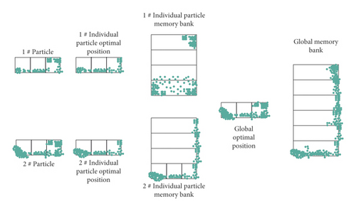
In the multi-objective particle swarm algorithm, the global memory bank is the Pareto optimal set to be formed eventually. After each particle update position, it is necessary to judge whether the new position can enter the individual memory bank and the global memory bank. For example, after updating the position of particle No. 1, it needs to be compared with each particle in the individual memory bank of No. 1 particle (the abovementioned example is an individual memory bank with 5 storage units, and at most 5 comparisons are required) to judge (the criterion for judgment is Pareto domination) whether the new position can enter the individual memory bank of particle 1. If it is possible to enter, it is necessary to further judge whether the individual memory bank of No. 1 particle is full. If it is not full, the particles enter directly. If it is full, it is necessary to judge the location of the particle again according to the corresponding criterion, and finally complete the update of the individual memory bank of No. 1 particle. We can find that in the process of updating the memory position of individual particles, each particle has to perform tedious comparison steps, and the tedious degree is determined by the size of the memory bank and the number of objective functions. After the update of the individual memory bank, the particles in the global memory bank should be compared in a similar way to complete the comparison of the global memory bank, and the comparison of the global memory bank is more complicated. The reason is that the capacity of the global memory bank is generally relatively large, and there are many particles stored, and it is also related to the total number of particles initialized. After updating the individual memory bank of all particles and the global memory bank of the whole group once, each particle position needs to be updated next time. The update process involves the update of the particle velocity, and the update of the particle velocity uses two storage units, the optimal position of the individual particle and the global optimal position of the population. Usually, the methods for obtaining the optimal position of individual particles and the global optimal position of the population are different, but they are both obtained by processing the particle positions in the individual memory bank and the global memory bank. It can be seen that the individual optimal position and the global optimal position in the multi-objective particle swarm optimization algorithm only play a guiding role in the speed update. The final solution is not stored in the global optimal position like the single-objective particle swarm optimization algorithm, but some noninferior solutions are stored in the global memory.
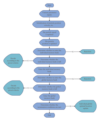
- (1)
Various pre-set parameters, including the number of particles, the number of iterations, the individual memory storage capacity, and the global memory storage capacity are input;
- (2)
Particle velocity, position, individual optimal position, global optimal position, individual memory bank, and global memory bank are initialized;
- (3)
The algorithm updates the particle velocity;
- (4)
The algorithm updates the position of each particle;
- (5)
The algorithm judges whether the updated particles can enter the individual memory bank according to the Pareto dominant condition. If the particle cannot, the particle is not retained. If the particle reaches the entry condition, the algorithm determines whether the individual memory bank is full. If the individual memory bank is not full, the particles go directly into the inventory. If the individual memory bank is full, it is necessary to decide whether or not to leave the particle according to preset criteria (such as the roulette method).
- (6)
The algorithm judges whether it can enter the global memory, and the selection method is the same as step (5);
- (7)
The algorithm judges whether the termination condition is satisfied. If the condition is met, the program terminates and the result is output. However, if the condition is not satisfied, the algorithm updates the individual global optimal position and goes to step (3).
Its flow chart is shown in Figure 2.
In order to facilitate the description of this method, the multi-objective problem here is selected as two objectives, as shown in Figure 3:
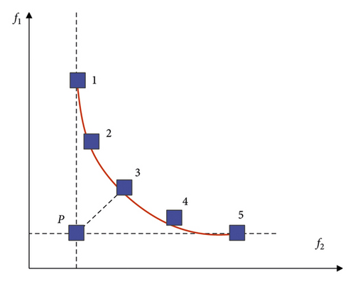
The horizontal and vertical axes are the two objective functions that need to be optimized for the multi-objective problem, respectively. The horizontal and vertical coordinates of the points in the f1 and f2 coordinate systems represent the optimized values of these two objective functions, respectively. Point P is the point formed by the two optimal results obtained by considering only the objective function f1 or f2 alone, that is, P(f2,min, f1,min) is the objective function f1 and f2 reaches the minimum solution at the same time. However, such a point does not exist in practical multi-objective optimization. Points 1 to 5 are points on the Pareto optimal Frontier, and point 1 is optimal for the objective function f2 but at the cost of sacrificing f1. Point 5 is optimal for f1 but very suboptimal for f2. In the geometric distance evaluation method, the point closest to point P is the compromise solution to be selected because it is the closest to the virtual ideal solution.
The ultimate goal of practical multi-objective solving problems in engineering applications is to solve a compromise solution suitable for engineering production. In order to obtain this compromise solution, the existing method is to form a Pareto optimal set first and then select it according to the needs in this optimal set. In order to avoid complicated comparisons and simplify the tedious steps of the program, this paper proposes a multi-objective particle swarm algorithm with virtual ideal particles. The algorithm no longer “runs and tires” in order to form a Pareto optimal set, but “reduces complexity and simplicity” directly to the goal. The basic principle is also relatively simple, that is, the distance from the ideal solution is used to judge the pros and cons of the particle position to determine the particle’s stay, as shown in Figure 4 below (two targets are still used here as an example).
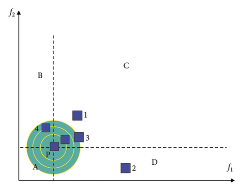
The point P(f1,min, f2,min) in Figure 4 has the same meaning as in Figure 3. It is a point formed by two minimum values obtained when only one objective function is considered alone, which is an idealized point. However, it is impossible to obtain such a point because of the mutual restrictive relationship when two practical goals are considered at the same time. The dotted line in the figure divides the first quadrant into four regions, A, B, C, and D. Among them, the A region is the region that cannot be optimized for the actual multi-objective problem, and the BCD is the region that can be optimized.
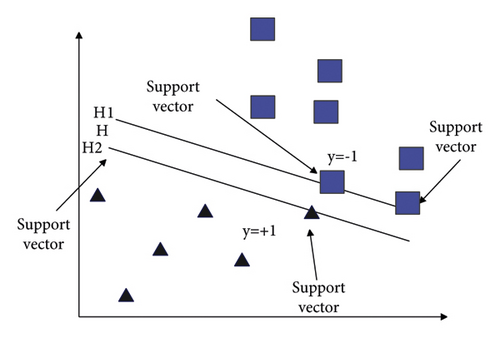
When the data is linearly separable in 2 dimensions, finding a plane that can maximize the area separating the two types of samples that are closest to each other is the simplest application of SVM in the case of classification. The abovementioned plane is defined as the optimal hyperplane, as shown in Figure 5.
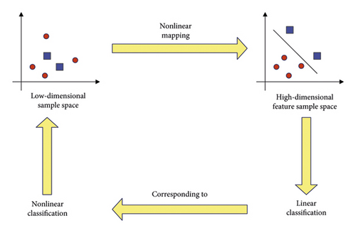
When faced with the data samples of practical problems, considering their linear inseparability, we need to construct a function to transform the original data and then map it into a high-dimensional space, and then we can construct the optimal classification hyperplane. Figure 6 shows the nonlinear mapping relationship between low-dimensional space and high-dimensional space.
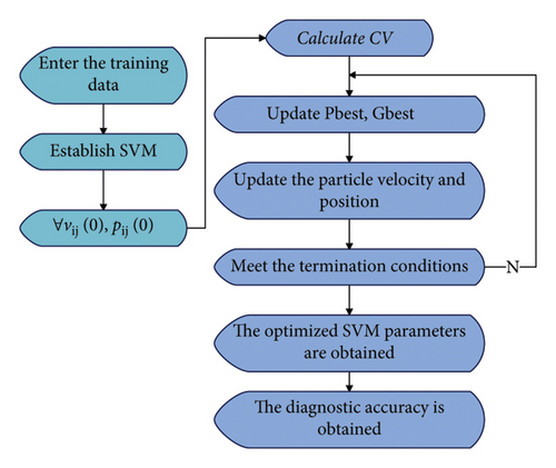
The parameters required to establish the support vector machine model mainly include the kernel function, the penalty factor C, and the width of the radial basis kernel function σ2. The radial basis kernel function has been selected for the kernel function, and now it is only necessary to find the optimal penalty factor C and the width of the radial basis kernel function σ2. If only relying on experiments to obtain the optimal parameters, its efficiency will be greatly reduced. At present, when the support vector machine finds the optimal parameters, the grid search method is usually used. However, this algorithm has the disadvantage of low optimization efficiency. This paper combines the PSO algorithm to optimize the twin support vector machine. Figure 7 below shows the optimized algorithm flow chart.
In the testing process, the parameters are selected, the population size is taken as 10, the number of iterations is taken as 100 times, and the program is terminated when the maximum number of iterations is reached. The convergence curve of the test function is obtained as shown in Figure 8.
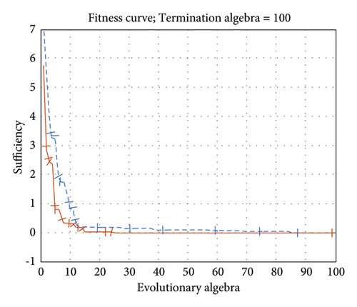
As shown in Figure 8, the solid line in the figure represents the improved particle swarm algorithm, and the dashed line represents the unimproved particle swarm algorithm. It can be seen from the fitness graph that the improved PSO algorithm can jump out of the local optimum and speed up the operation speed of the algorithm. That is, the convergence speed becomes faster, and the improved PSO algorithm is more accurate than the unimproved PSO algorithm. Therefore, it is proved that the improved PSO algorithm used in this paper has certain practical significance.
On this basis, the application effect of the PSO-optimized twin support vector machine in the medium and long-term load forecasting of the new normal economy is verified, and the results shown in Figure 9 are obtained through cluster analysis.
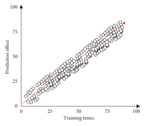
Through the abovementioned experimental studies, it is verified that the PSO-optimized twin support vector machine has a very good application effect in the medium and long-term load forecasting under the background of a new normal economy.
3. Conclusion
Under the background of the new normal of the economy, with the changes in the economic growth environment, there are also new requirements for the economic growth model, and the economic growth model has changed from factor-driven to innovation-driven. Under the factor-driven growth model, the most important thing for enterprise development is to obtain the corresponding factor resources such as land, capital, and talents. However, under the innovation-driven growth model, what enterprises need most for development is an institutional environment that is conducive to intellectual property protection, conducive to stimulating innovation, conducive to obtaining high-level capital, and conducive to fair competition. In this paper, the twin support vector machine optimized by PSO is used to construct a medium and long-term load forecasting model under the background of the new normal economy, which provides a better forecasting effect for subsequent economic development. The experimental study verifies that the PSO-optimized twin support vector machine has a very good application effect in medium and long-term load forecasting under the background of the new normal economy [20].
Conflicts of Interest
The authors declare no conflicts of interest.
Acknowledgments
This work was supported by Nanchang Institute of Science and Technology Humanities And Social Sciences Research Project “Research on securitization of plant variety rights from the perspective of grain storage and technology” (NGRW-21-06). “Jiangxi Observation Report” subject and key project of social science planning of Jiangxi Province in 2022, tracking research on building a model place for Rural Revitalization in the new era in Jiangxi, (22SQ06) 2018 decision support collaborative innovation center project for the sustainable development of modern agriculture and its advantageous industries in Jiangxi, research on the measurement and improvement of China’s agricultural total factor productivity, (2018B02).
Open Research
Data Availability
The labeled dataset used to support the findings of this study is available from the corresponding author upon request.


