Music education should pay attention to popular music that exists in students’ real life and deeply affects them. Moreover, it needs to be combined with “popular classical music” to make them happily learn popular music, appreciate popular music artistically, and feel popular music aesthetically. This study combines the audio frame feature recognition technology to evaluate the effect of multimedia popular music teaching and improve the quality of multimedia popular music teaching. Moreover, this study adaptively revises the speech spectrum technology to construct a multimedia pop music system based on audio frame feature recognition technology. Finally, this study verifies the performance of this system through experimental research. According to the results of experimental research, it can be seen that the effect of the system proposed in this study is very good.

1. Introduction

The composition of music art should be diverse, including both traditional music and modern music, and other mainstream and nonmainstream forms of music. Therefore, since we can attach importance to classical music and traditional music, we must also attach importance to modern music and popular music. Most popular music is passionate, full of emotions, sentimental, or happy and enmity, and it is always based on the principle of depicting and adapting to the public’s psychology to the maximum. In addition, it should be noted that the appreciation of popular music also requires some kind of artistic guidance and the artistic imagination of the audience. The need for spirit is the essence of popular music. Although popular music is as vast as a sea of smoke, it will always leave something shining after the big waves wash the sand. It will become classic and inspiration [1].

At present, our country is in a period of rapid development, and our society is in a period of transformation. Students living in such an era are facing heavy learning pressure on the one hand and are in a psychologically sensitive period on the other hand. They are in a special growth stage of transition from immaturity to maturity. Compared with the previous childhood and later adulthood, the psychology of this period has the characteristics of poor stability, high emotionality, high sentimentality, and strong sensitivity [2]. Popular music has a distinctly popular character. Most of its content is close to the lives of ordinary people and expresses the feelings of ordinary people. Today, popular music has become the mainstream music culture of the society. For teenagers, it is obviously different from children’s songs, and it has the atmosphere of the times, which can resonate with their own hearts. Moreover, popular music occupies an important part in the lives of college students [3].

This study combines audio frame feature recognition technology to evaluate the effect of multimedia popular music teaching, improve the quality of multimedia popular music teaching, improve the role of popular music in the growth of students, and promote the healthy development of students’ body and mind.

2. Related Work

Due to the rapid development of computer technology and informatics, and people’s demand for fast and effective audio recognition, audio recognition demonstrations using audio frame recognition have been widely used. Literature [4] laid a theoretical basis for the audio frame recognition technology. Literature [5] found a speech spectrogram and can automatically depict this spectrogram. People think that everyone’s fingerprints are different from each other, and it usually takes millions of people to find almost identical fingerprints. The same should be true for audio frames [6]. Literature [7] obtained a method based on pattern matching and probability statistical analysis to support the development of audio frame recognition technology. Many scholars paid attention to this, which pushed the audio frame recognition to a peak. During this period, everyone focuses on the feature extraction direction. Literature [8] proposed the UBM-MAP (Universal Background Model-Maximum Posterior Probability) structure in the speaker verification task, which made the audio frame recognition from the laboratory to the practical. Important contribution: UBM-MAP reduces the dependence of the statistical model GMM on the training set. When training the model, only a few sentences of the speaker are needed, so it is relatively simple and flexible to use, and its accuracy is relatively high. Subsequently, the support-vector machine (SVM) technology was introduced into the audio frame recognition and achieved good results [9].

Although there have been many matching algorithms such as GMM-SVM, the effect is not as good as GMM and GMM-UBM [10]. Under the current development trend, audio frame recognition has gradually moved from the original laboratory stage to the practical stage. When in a pure voice environment, the audio frame recognition rate can reach a high accuracy rate, but when in a noisy environment, it will reduce the accuracy rate a lot, so now noise has become one of the main reasons that affect the recognition performance. Therefore, the research on noise suppression algorithms is urgent. Among them, the speech enhancement technology is produced in this environment, and its purpose is to extract pure speech signals from noisy speech as much as possible [11]. Literature [12] proposed the use of spectral subtraction to eliminate noise; literature [13] studied Wiener filtering algorithms for noise removal. These algorithms based on short-time spectrum estimation are suitable for environments with relatively large signal-to-noise ratios, and the algorithm is simple and easy to implement, so it has always had a strong vitality, and many people still use it.

Due to the vigorous development of very large-scale integrated (VLSI) circuit technology, the possibility of real-time implementation of voice enhancement is provided. Literature [14] published an algorithm for soft decision noise removal; literature [15] applied the Kalman filter to speech denoising. However, these traditional various filters are processed by spectrum analysis technology, which is a method of using Fourier transform to map the signals one by one into the frequency domain and then analyze them. This method will only work when the selected signal is stable and the spectral characteristics are obviously different from the noise, but in real life people often encounter unstable signals, and the frequency band of the signal and the frequency band of the noise tend to overlap together, so traditional methods are becoming less and less satisfactory. The rapid development of mobile communication technology has given a realistic impetus to the research of speech enhancement technology. For example, wavelet decomposition technology [16] is proposed for speech signals with noise. This method is formed with the mathematical analysis method of wavelet decomposition. It is a time-domain and frequency-domain analysis with multiresolution characteristics. Because of this, the local characteristics of the signal can be combined with the time domain and frequency domain. This feature is superior in the analysis of nonstationary signals. At the same time, it also combines part of the theoretical basis of spectral subtraction, which is now the focus of multidisciplinary attention. But there is a weak point in wavelet denoising, that is, the energy of noise needs to be estimated, but people often do not know what noise is there. Therefore, the independent component analysis method [17] has been developed. Its central idea is to combine a set of observation signals linearly mixed from source signals (such as pure speech and noise), assuming that the source signals are independent of each other in time. The algorithm separates the source signal, and the signal and noise meet this point. This method does not need to understand the noise characteristics.

3. Audio Frame Feature Recognition Algorithm Model

Adaptive postfiltering is a technique that adaptively corrects the speech spectrum according to the spectral characteristics of the local speech in order to improve the quality of the synthesized speech. In order to essentially understand the principle of adaptive postfiltering in speech coding, it is explained in terms of Wiener filtering and the hearing model of the human ear.

A very important element of signal processing is to extract the signal from the noise or to suppress the companion noise to the maximum extent possible. One effective way to achieve this is to design a filter with optimal linear filtering characteristics.

The classical Wiener filter describes how to design the best filter for noise suppression: determine the system function H(z) of the filter so that the mean square error (MSE) between the filtered output signal and the original signal is minimized. We assume that the energy spectral density of the signal is S(w), the spectral density of the independent additional noise is H(w), and the frequency response of the optimal filter should be [18]

(1)

From formula (1), it can be seen that the gain of the filter is close to 1 at frequencies with a large signal-to-noise ratio (SNR). At frequencies with smaller SNR, the gain of the filter is correspondingly smaller. The postfilter of the conventional narrowband encoder is usually applied to the synthesized speech at the decoding end, as shown in Figure 1.

Details are in the caption following the image — Open in figure viewer PowerPoint

The ideal short-time postfilter has a frequency response that is similar to the spectral envelope of the speech signal. In the linear predictive encoder, the frequency response of the LPC synthesis filter is similar to the spectral envelope of the input speech signal. Therefore, the expression of the transfer function of the short-time postfilter is generally [19]

(2)

Among them, is the transfer function of LPC predictor coefficients, a_i is the LPC predictor coefficients, p is the order of LPC predictor, and the corresponding transfer function of the LPC synthesis filter is 1/(1-A(z)). The scale factor γ corrects the LPC synthesis filter as shown in Figure 2.

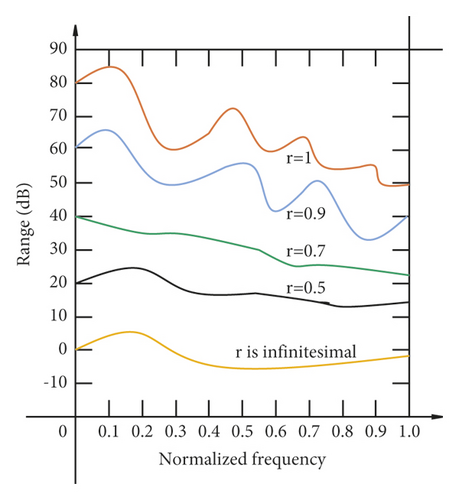
If 1 − A(z/β) is used only as a short-time postfilter, it reduces noise, but it introduces a spectral skew with a low-pass effect, which can lead to a “muffled” sound. Therefore, a corresponding zero-point filter 1 − A(z/β) is introduced to reduce the spectral skew.

Thus, the frequency response of the short-time postfilter H(z) is as follows:

(3)

From formula (3), it can be seen that, in the logarithmic domain, the frequency response of H(z) is the difference between the frequency responses of the two weighted LPC synthetic filters so that some of the skews can be removed, as shown in Figure 3.

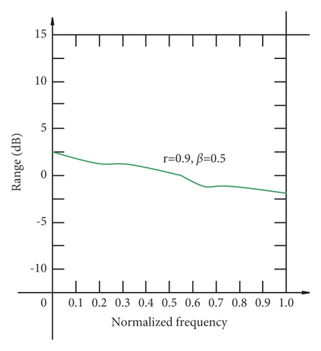
Usually, in order to further reduce the low-pass effect, a first-order filter with a transfer function of 1 − μz⁻¹ can be added to cascade with a short-time postfilter.

The long-time postfilter is introduced to weaken the staccato rate component between the fundamental tones without introducing spectral skew. The transfer function of the long-time postfilter with zero and pole is [20]

(4)

Among them, G is the adaptive gain factor, p is the fundamental period, and 0 < λ < 1,0 < γ < 1.

The phases of the p poles of H(z) are 0, 2π/p, 4π/p, …, (p − 1)2π/p, corresponding to the peaks of the harmonics of the fundamental tone in turn. The phases of the p zeros of H(z) are π/p, 3π/p, …, (2p − 1)π/p, corresponding to the troughs between the harmonics of the fundamental, respectively. γ and λ vary with the clearness of the speech, thus controlling the degree of long-time postfiltering according to the periodicity of the speech.

The adaptive gain G is very important for the long-time postfilter. For clear or most consonants, usually γ and λ are 0, that is, there is no long-time postfilter. If G = 1, the energy of the speech signal after long-time postfiltering is equal to the energy before filtering. For stable turbid tones, if G = 1, the energy of the signal is amplified after the long-time postfilter. This is because according to formula (5), each current fundamental tone cycle waveform is superimposed on the previous fundamental tone cycle waveform.

(5)

This leads to different effects of the postfilter power gain on the clear and turbid tones, making the volume of the clear tones decrease relative to the turbid tones, and thus, the speech quality is impaired. A derivation is given as follows:

(6)

The full polar part (denominator part) of the transfer function in formula (3) corresponds to the recursive infinite impact response (IIR) filtering operation. Its impact extends to future frames, and the full-zero part (numerator part) corresponds to the nonrecursive FR filtering operation, and its impact basically stays in the current frame. Therefore, in practical applications, a very small λ value is generally chosen, or even λ = 0. In this postfilter design of the wideband embedded speech encoder, the long-time postfilter used is the filter with no poles.

For an analytic-synthetic encoder like the CELP-based model, the optimal excitation parameters are searched in the perceptually weighted domain, obtained by minimizing the minimum mean square error between the input speech and the synthesized speech.

The perceptually weighted filter for a conventional narrowband signal is [21]

(7)

Among them, A^′(z) is the linear prediction coefficient, and γ₁ and γ₂ are the control factors. In this way, the quantized noise (usually assumed to be white noise) is weighted by 1/W^′(z), which also shapes the noise spectrum to have a resonant peak spectrum similar to the input speech signal.

However, traditional perceptually weighted filters for narrowband signals do not exhibit large spectral tilts. For broadband signals, the dynamic range between low and high frequencies is very large, and the spectral tilt is also very large, which requires the perceptually weighted filter to represent not only the resonant peak structure but also the spectral tilt. Therefore, the perceptual weighting of the broadband signal should be decomposed. First, the input signal is pre-emphasized, that is, the high-frequency part is raised by pre-emphasizing the filter P(z) = 1 − μz⁻¹. Then, LPC prediction coefficients are calculated with the transfer function A(z). Finally, the perceptually weighted filter is obtained, as shown in the following formula:

(8)

A(z) is calculated on the basis of the pre-emphasized signal, so the tilt of 1/A(z/γ₁) is smaller than the A(z) directly calculated on the input speech. At the same time, the synthesized speech has to be de-emphasized at the decoding end, that is, by 1/P(z). In this way, the spectral correction of the quantization error is W⁻¹(z)P⁻¹(z), that is, 1/A(z/γ₁).

Although the noise spectrum is suppressed according to 1/A(z/γ₁) shaping, the experiments show that there is still subtle noise in the synthesized speech, especially in the low code rate case, so it is necessary to introduce the postfiltering design at the decoding end.

Therefore, if the object of long-time postfiltering is the prediction error signal, it is better than the object of the speech signal. Moreover, the calculation of the control factor in the long-time postfilter is related to the turbidity of the speech, so the control factor can be calculated in the residual signal domain to obtain more accurate values.

The postfilter design in G729 proves the correctness of this idea. The synthesized speech is first passed through the short-time predictor to obtain the residual signal; then, the long-time postfilter is applied to this residual signal, and finally, the short-time postfilter is applied.

Figure 4 shows the postprocessing flowchart of this wideband embedded encoder, and the modules are described in detail in the following.

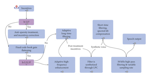
The antisparse processing is performed only at the rate of 8 kb/s, and it acts on the fixed codebook vector with the purpose of improving the low bit rate perception quality. This is because if only 8kb/s streams are received at the decoder, the fixed codebook vector has only three nonzero sample points per subframe (called “sparse”), and this sparsity causes subjective auditory unrealism. In order to reduce the artificial perception of this sparsity, antisparse processing is applied to the surrogate digital book vector.

The smoothing of the fixed codebook gain is processed based on two parameters, the turbidity and smoothness of the speech. The turbidity of the speech is estimated as follows:

(9)

E_v and E_c are the energy of adaptive codebook and fixed codebook, respectively, , and . The closer λ is to 0, the closer the frame is to pure turbid speech. The closer λ is to 1, the closer the frame is to pure clear speech.

The stability factor θ is estimated by using the distance Ds between the ISP coefficients of the current frame (ISP is the frequency pair of the conduction spectrum, which is the frequency-domain representation of the LPC coefficients) and the ISP coefficients of the past frames [22]:

(10)

Among them, p is the order of the line prediction coefficient, ispn is the ISP coefficient of the current frame, and ispn-1 is the ISP coefficient of the previous frame. The closer Q is to 1, the more stable the frame is.

Considering the comprehensive turbidity and stability, the smoothing control factor Sm can be defined as follows:

(11)

That is, if Sm is close to 1 then it indicates a smooth nonturbulent signal, such as smooth background noise. The smoothing process for a fixed codebook gain is as follows:

(1)
If the fixed codebook gain , the algorithm calculates and then compares tmp with . If , the algorithm sets tmp to . Its initial value of is 0.
(2)
If the fixed codebook gain , the algorithm calculates tmp = 0.84 and then compares tmp with . If , the algorithm sets tmp to .
(3)
The algorithm updates , that is, the algorithm sets up .
(4)
Finally, the smoothed fixed codebook gain is obtained: .

The fixed codebook describes the details of speech, and the energy is mainly concentrated in the high-frequency part, and the low-frequency part has less energy. For pure turbid speech, adjusting the energy of the fixed codebook in low and high frequencies within a reasonable range can improve the perception of speech. The encoder uses high-frequency enhancement filters to enhance the first and second layers, as shown in Figure 5.

The high-frequency enhancement filter is a high-pass filter whose coefficients c_pe can be adaptively adjusted according to the turbidity of speech. c_pe = 0.125(1 + r_v), r_v = (E_v + E_c), and E_V and E_C are the energy of adaptive codebook and fixed codebook, respectively. When the turbidity is larger (that is, C_pe = 0.25), the higher frequency is enhanced and the lower frequency is weakened. The high-frequency enhancement filter expression is shown as follows:

(12)

The fixed codebook is passed through this filter to get a new fixed codebook:

(13)

In turn, the total synthetic excitation exc2(n) is calculated according to formula (14), and among them, v(n) adaptive codebook, for

that is the adaptive codebook gain,

is the fixed codebook, and Liang is the fixed codebook gain.

(14)

The long-time postfilter of this encoder is designed using the idea of a conventional long-time postfilter. The purpose of applying it to the excitation is to eliminate the noise between the excitation harmonics. Figure 6 shows an example of a long-time postfilter with the following expression:

(15)

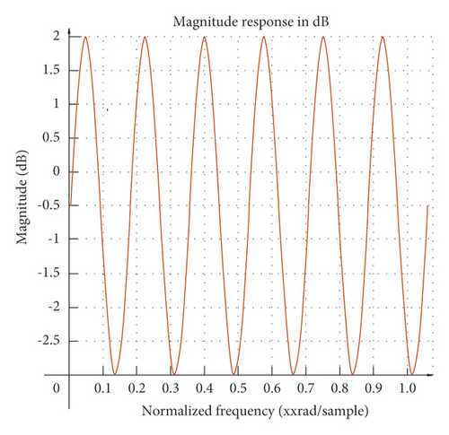
T is the integer fundamental delay of the current subframe. r = 0.5. G is the adaptive control factor, and 0 < g < 1, which allows adaptive control of the long-time postfilter, which is expressed as follows: if the current subframe excitation is strongly correlated with past excitations (for example, a clear tone), g tends to 1. Conversely, if the current subframe excitation is weakly correlated with past excitations (for example, a clear tone), g tends to 0, that is, it does not pass the long-time postfilter. The values of T and g are calculated by the following procedure.

Here, the selection of T is very important because it determines the harmonic period of the long-time filter, so it has to be refined. First, the best integer fundamental delay T₁ is selected in the range [(T₀ − 1), (T₀ + 1)], where T₀ is the integer fundamental delay of the current subframe. By calculating the autocorrelation R(k) of the current subframe excitation r(n) and the delayed excitation r(n − k) (as in formula (16)), the one with the maximum R(k) is the best integer fundamental delay T₁.

(16)

The best fractional fundamental delay T is then selected. t is chosen around T₁ with an accuracy of 1/8. The algorithm then calculates R^′(k) (as in formula (17)) so that the maximum is the best fundamental delay T.

(17)

Among them, r(n) is the current subframe excitation and r_k(n) is the excitation code vector obtained by interpolating around T₁. r_k(n) is first obtained by an interpolation filter of length 33, and after finding the optimal fractional fundamental delay T, r_k(n) is then rederived by an interpolation filter of length 129. When the R(k) calculated by the filter of length 129 is larger than the Z obtained by the filter of length 33, the filter of length 129 is chosen.

When the optimal fundamental delay T is found, the normalized autocorrelation is obtained by dividing R(T) by the sum of the squares of r(n). If the normalized autocorrelation is less than 0.5, as in formula (18), then g = 0, which is equivalent to the excitation not passing through the long-time filter. That is, when the correlation between the excitation of the frame and the past excitation is small, the long-time filter is not passed.

(18)

The gain coefficient g is calculated by the following equation:

(19)

The core layer of this embedded encoder is the CELP model. At the same time, it is necessary to be able to handle both wideband speech (bandwidth 50–7000 Hz) and narrowband speech (bandwidth 300–4000 Hz). In order to improve the quality of synthesized speech for these two types of input speech, this study tries to introduce the traditional short-time postfilter.

The purpose of applying the short-time postfilter to the synthesized speech is to attenuate the noise between the resonance peaks. The expressions are as follows:

(20)

Among them,

is the quantized linear prediction filter. It is experimentally concluded that the short-time postfiltering performs best when the control factors r₁ = 0.6 and r₂ = 0.7. The control factor also shows that the short-time postfiltering for wideband speech cannot be too strong (usually, the control factors of short-time postfiltering in narrowband speech encoders are r = 0.5 and r = 0.8). If it is assumed that hf(n) is the impulse response of

, the gain gf is calculated from h(n) as in formula (21):

(21)

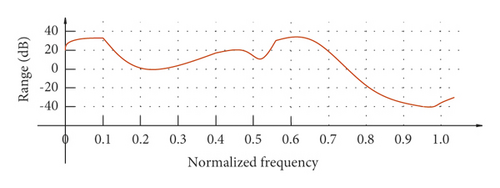
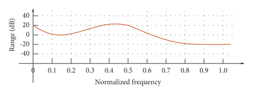
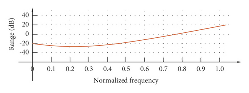
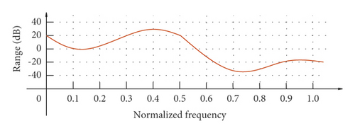
Figure 7(a) shows the frequency response of the synthesis filter for one-frame speech and (b) shows the frequency response of . It can be seen from the figure that (b) can track the resonance peaks of the speech spectrum and weaken the energy between the resonance peaks, but this filter introduces a spectral tilt. By adding the spectral tilt compensation filter, the spectral tilt of the filter after a short time is reduced, as shown in Figure (c). So the synthesized speech has to undergo spectral tilt compensation and adaptive gain control after entering the short-time filter, and these three modules are one and the same.

The filter Ht(z) is used to compensate for the skew of the short-time postfilter, and the expression is as follows:

(22)

Here, is the skew factor and . r is a constant, r, = 0.9 when , and ri = 0.2 when .

The purpose of an adaptive gain control is to compensate for the energy difference between the synthesized speech s(n) before filtering and the filtered speech sf(n). The gain adjustment factor is calculated as follows:

(23)

The gain-adjusted speech sf'(n) is as follows:

(24)

The initial value of g⁽ⁿ⁾ is g⁽⁻¹⁾ = 1, and then, it is updated point by point:

(25)

For a given input signal x(n), if we want to obtain an output with a sampling rate of LM times, the method is to interpolate x(eight) by L times, pass it through a low-pass filter h(n), and then extract it by M times. The frequency response of the low-pass filter h(n) is expressed as follows:

(26)

Among them, ω_x is the normalized cutoff frequency, and C is a constant in the equation, which is the calibration factor and should be taken as C-L. The LM time sampling rate conversion equation is as follows:

(27)

Among them, K=N/L, N is the length of the filter h(n), 〈nM〉_L denotes the remainder of nML, and ⌊nM/L⌋ denotes rounding to nM/L.

(1)
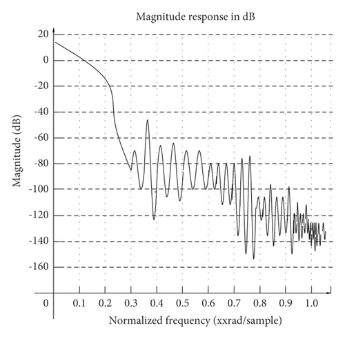
Algorithm performs downsampling from 16 kHz to 12.8 kHz. We set L = 4, M = 5, that is, 4/5 downsampling, and after conversion, the sampling rate is 12.8 kHz, that is, each frame of speech from 320 sample points to 256 sample points. The normalized cutoff frequency o for h(n) is 0.2 n, the length is N = 120, and the amplitude response is shown in Figure 8.
(2)
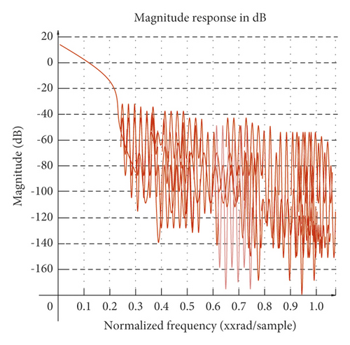
Algorithm performs upsampling from 8 kHz to 12.8 kHz. We set up L = 8, M = 5, that is, 8/5 upsampling, and the converted sampling rate is 12.8 kHz, that is, each frame of speech changes from 160 sample points to 256 sample points. The normalized cutoff frequency ω_x of h(n) is 0.125π, the length is N = 256, and the amplitude-frequency response is shown in Figure 9.
(3)
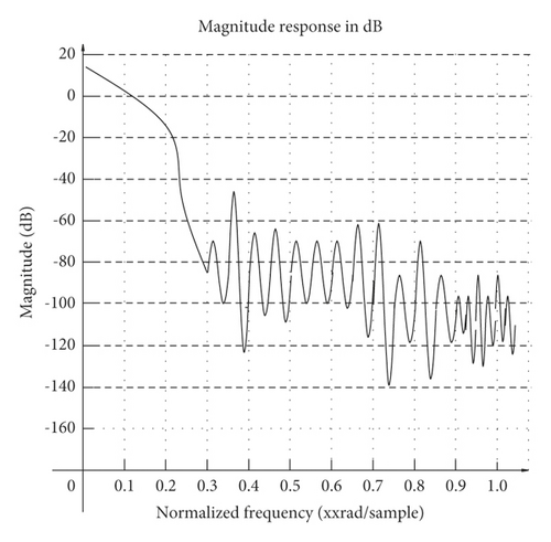
Algorithm performs upsampling from 12.8 kHz to 16 kHz. The 4/5 upsampling is performed, and the converted sampling rate is 16 kHz, which means that each frame of speech changes from 256 sample points to 320 sample points. The amplitude response is shown in Figure 10, where L = 5, M = 4, h(n) normalized cutoff frequency ω_x is 0.2π, and the length is N-120.
(4)
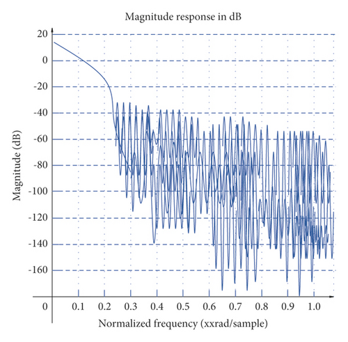
Algorithm performs downsampling from 12.8 kHz to 8 kHz. The 5/8 downsampling is performed on the speech signal with a 12.8 kHz sampling rate, and the converted sampling rate is 8 kHz, which means that each frame of speech changes from 256 sample points to 160 sample points. Among them, L = 5, M = 8, h(n) normalized cutoff frequency ω_x is 0.125π, the length is N = 240, and amplitude-frequency response normalized cutoff frequency is shown in Figure 11.

4. Evaluation of Multimedia Popular Music Teaching Effect Based on Audio Frame Feature Recognition

The music teaching system provides a variety of music learning services, online guidance, virtual environment learning, and intelligent evaluation. In order to realize its functions, the entire platform adopts a five-layer architecture, and from bottom to top, they are as follows: access layer, data processing layer, data storage layer, scene management layer, and application layer, as shown in Figure 12.

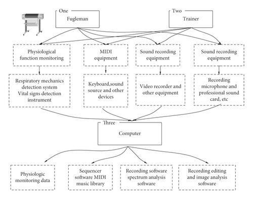
The system builds a corresponding database for students. Based on the traditional teaching experience, this study does a quantitative analysis of the teaching content at all levels. The statistical analysis and results of a large number of data can provide more powerful reference data for the teaching and training of teachers and students. The framework of the external facilities and equipment of the system is shown in Figure 13.

The audio frame feature recognition effect and teaching effect of the system proposed in this study are evaluated, and the results shown in Tables 1 and 2 below are obtained.

1. Audio frame feature recognition effect.

No.	Audio frame recognition
1	92.44
2	93.31
3	94.62
4	94.72
5	90.97
6	91.16
7	95.15
8	91.18
9	93.39
10	89.98
11	95.92
12	89.06
13	90.93
14	94.99
15	94.61
16	95.25
17	95.39
18	95.00
19	94.88
20	93.30
21	92.34
22	91.24
23	90.44
24	90.26
25	94.89
26	90.11
27	95.04
28	92.59
29	91.64
30	94.67
31	94.68
32	93.94
33	95.77
34	94.49
35	95.73
36	89.39

2. Multimedia popular music teaching effect.

No.	Teaching effect
1	88.07
2	85.26
3	89.39
4	89.74
5	87.39
6	82.90
7	84.06
8	89.92
9	94.00
10	85.92
11	90.00
12	91.31
13	85.73
14	92.34
15	89.48
16	82.45
17	89.44
18	89.01
19	83.84
20	89.57
21	92.83
22	89.29
23	84.02
24	86.10
25	91.00
26	90.01
27	88.85
28	83.34
29	91.33
30	92.88
31	91.33
32	85.89
33	83.57
34	89.03
35	89.03
36	85.95

It can be seen from the above research that the multimedia popular music system based on audio frame feature recognition technology proposed in this study has good results, so the multimedia popular music system based on audio frame feature recognition technology can be practiced in actual teaching later.

5. Conclusions

Popular music is diversified, some are suitable for college students to appreciate, and some should really be kept away from college students. It is precisely because of this uneven development of popular music that as educators always worry that young students will be harmed, so they have an attitude of rejecting popular music. However, in the context of the entire society, this kind of educational rejection will not reduce the impact of popular music on college students. In the past, the theoretical circles’ rejection and criticism of popular music were somewhat influenced by the opposition between Eastern and Western ideologies. They subconsciously think that as long as they are imported from the West, they are corrupt and bad. Popular music is purely westernized regardless of its origin or its own content and form. Therefore, as a socialist country, we should resist it and protect young people from this decadent culture. Before the reform and opening up, this recognition lasted for a long time. This study combines audio frame feature recognition technology to evaluate the effect of multimedia popular music teaching, improve the quality of multimedia popular music teaching, improve the role of popular music in the growth of students, and promote the healthy development of students’ body and mind.

Conflicts of Interest

The author declares no competing interests.

Acknowledgments

This study was sponsored by the Shandong University of Arts.

Open Research

Data Availability

The labeled dataset used to support the findings of this study is available from the corresponding author upon request.

References

1 Dash D., Farooq R., Panda J. S., and Sandhyavani K. V., Internet of Things (IoT): the new paradigm of HRM and skill development in the fourth industrial revolution (industry 4.0), The IUP Journal of Information Technology. (2019) 15, no. 4, 7–30.
Google Scholar
2 Chin J., Callaghan V., and Allouch S. B., The Internet-of-Things: r, Journal of Ambient Intelligence and Smart Environments. (2019) 11, no. 1, 45–69, https://doi.org/10.3233/ais-180506, 2-s2.0-85060956029.
10.3233/AIS-180506
Web of Science® Google Scholar
3 Bedi G., Venayagamoorthy G. K., Singh R., Brooks R. R., and Wang K. C., Review of internet of things (IoT) in electric power and energy systems, IEEE Internet of Things Journal. (2018) 5, no. 2, 847–870, https://doi.org/10.1109/jiot.2018.2802704, 2-s2.0-85041551917.
10.1109/JIOT.2018.2802704
Web of Science® Google Scholar
4 Bisio I., Delfino A., Grattarola A., Lavagetto F., and Sciarrone A., Ultrasounds-based context sensing method and applications over the internet of things, IEEE Internet of Things Journal. (2018) 5, no. 5, 3876–3890, https://doi.org/10.1109/jiot.2018.2845099, 2-s2.0-85048160210.
10.1109/JIOT.2018.2845099
Web of Science® Google Scholar
5 Chamberlain A., Bødker M., Hazzard A., and McGookin D. K., Audio technology and mobile human computer interaction, International Journal of Mobile Human Computer Interaction. (2017) 9, no. 4, 25–40, https://doi.org/10.4018/ijmhci.2017100103, 2-s2.0-85028035874.
10.4018/IJMHCI.2017100103
Google Scholar
6 Kiliç D. B. Ç., Pre-service music teachers’ metaphorical perceptions of the concept of a music teaching program, Journal of Education and Learning. (2017) 6, no. 3, 273–286.
10.5539/jel.v6n3p273
Google Scholar
7 Hoffman D. L. and Novak T. P., Consumer and object experience in the internet of things: an assemblage theory approach, Journal of Consumer Research. (2018) 44, no. 6, 1178–1204, https://doi.org/10.1093/jcr/ucx105, 2-s2.0-85040119972.
10.1093/jcr/ucx105
Web of Science® Google Scholar
8 Jia B., Hao L., Zhang C., Zhao H., and Khan M., An IoT service aggregation method based on dynamic planning for QoE restraints, Mobile Networks and Applications. (2019) 24, no. 1, 25–33, https://doi.org/10.1007/s11036-018-1135-7, 2-s2.0-85054484692.
10.1007/s11036-018-1135-7
Web of Science® Google Scholar
9 Waldron J., Mantie R., Partti H., and Tobias E. S., A brave new world: theory to practice in participatory culture and music learning and teaching, Music Education Research. (2018) 20, no. 3, 289–304, https://doi.org/10.1080/14613808.2017.1339027, 2-s2.0-85021639330.
10.1080/14613808.2017.1339027
Web of Science® Google Scholar
10 Zhang J. and Tao D., Empowering things with intelligence: a survey of the progress, challenges, and opportunities in artificial intelligence of things, IEEE Internet of Things Journal. (2021) 8, no. 10, 7789–7817, https://doi.org/10.1109/jiot.2020.3039359.
10.1109/jiot.2020.3039359
Web of Science® Google Scholar
11 Gun E., The opinions of the preservice music teachers regarding the teaching of orchestra and chamber music courses during distance education process, Cypriot Journal of Educational Sciences. (2021) 16, no. 3, 1088–1096.
10.18844/cjes.v16i3.5827
Google Scholar
12 Muhammad G., Rahman S. M. M., Alelaiwi A., and Alamri A., Smart health solution integrating IoT and cloud: a case study of voice pathology monitoring, IEEE Communications Magazine. (2017) 55, no. 1, 69–73, https://doi.org/10.1109/mcom.2017.1600425cm, 2-s2.0-85010053609.
10.1109/MCOM.2017.1600425CM
Web of Science® Google Scholar
13 Shengmin X., Analysis on the innovative strategy of national music teaching in colleges from the perspective of visual communication, Studies in Sociology of Science. (2017) 7, no. 6, 52–55.
Google Scholar
14 Lian Z., Research on aesthetic education in instrumental music teaching, Journal of Literature and Art Studies. (2020) 10, no. 5, 435–439, https://doi.org/10.17265/2159-5836/2020.05.008.
10.17265/2159-5836/2020.05.008
Google Scholar
15 Kim S. K., Sahu N., and Preda M., Beginning of a new standard: internet of media things, KSII Transactions on internet and information systems. (2017) 11, no. 11, 5182–5199.
Web of Science® Google Scholar
16 Kaplan A. and Haenlein M., Siri, Siri, in my hand: w, Business Horizons. (2019) 62, no. 1, 15–25, https://doi.org/10.1016/j.bushor.2018.08.004, 2-s2.0-85055962995.
10.1016/j.bushor.2018.08.004
Web of Science® Google Scholar
17 Reyes F. L., A community music approach to popular music teaching in formal music education, The Canadian Music Educator. (2017) 59, no. 1, 23–29.
Google Scholar
18 Jones V. K., Voice-activated change: marketing in the age of artificial intelligence and virtual assistants, Journal of Brand Strategy. (2018) 7, no. 3, 233–245.
Google Scholar
19 Aithal P. S. and Aithal S., Management of ICCT underlying technologies used for digital service innovation, International Journal of Management, Technology, and Social Sciences. (2019) 4, no. 2, 110–136, https://doi.org/10.47992/ijmts.2581.6012.0077.
10.47992/IJMTS.2581.6012.0077
Google Scholar
20 Johnson C., Teaching music online: changing pedagogical approach when moving to the online environment, London Review of Education. (2017) 15, no. 3, 439–456, https://doi.org/10.18546/LRE.15.3.08, 2-s2.0-85042645878.
10.18546/LRE.15.3.08
Google Scholar
21 Phylis Lan Lin P. L., Trends of internationalization in China’s higher education: opportunities and challenges, US-China Education Review B. (2019) 9, no. 1, 1–12, https://doi.org/10.17265/2161-6248/2019.01.001.
10.17265/2161-6248/2019.01.001
Google Scholar
22 Hong S. Y. and Hwang Y. H., Design and implementation for iort based remote control robot using block-based programming, Issues in Information Systems. (2020) 21, no. 4, 317–330, https://doi.org/10.48009/4_iis_2020_317-330.
10.48009/4_iis_2020_317-330
Google Scholar

Citing Literature

All articles

Evaluation of Multimedia Popular Music Teaching Effect Based on Audio Frame Feature Recognition Technology

Abstract

1. Introduction

2. Related Work

3. Audio Frame Feature Recognition Algorithm Model

4. Evaluation of Multimedia Popular Music Teaching Effect Based on Audio Frame Feature Recognition

5. Conclusions

Conflicts of Interest

Acknowledgments

Open Research

Data Availability

References

Citing Literature

Figures

References

Information

About Wiley Online Library

Help & Support

Opportunities

Connect with Wiley