Exploring the influencing factors of intercity travel mode choice can reveal passengers’ travel decision mechanisms and help traffic departments to develop an effective demand management policy. To investigate these factors, a survey was conducted in Xi’an, China, to collect data about passengers’ travel chains, including airplane, high-speed railway (HSR), train, and express bus. A Bayesian mixed multinomial logit model is developed to identify significant factors and explicate unobserved heterogeneity across observations. The effect of significant factors on intercity travel mode choice is quantitatively assessed by the odds ratio (OR) technique. The results show that the Bayesian mixed multinomial logit model outperforms the traditional Bayesian multinomial logit model, indicating that accommodating the unobserved heterogeneity across observations can improve the model fit. The model estimation results show that ticket purchasing method, comfort, punctuality, and access time are random parameters that have heterogeneous effects on intercity travel mode choice.

1. Introduction

The high-speed railway (HSR) plays an increasingly key role in intercity transportation because of its time advantages over conventional trains (which we refer to as trains) and low prices compared with airplanes. It also has the merits of punctuality, comfort, and low energy cost [1]. The HSR network in China has experienced rapid growth, with a total length of 35,000 km in 2019, accounting for more than two-thirds of the global HSR network [2, 3]. According to the long-term railway network plan, a grid of eight vertical and eight horizontal HSR lines will be in operation across 80% of the megacities in China by 2020 [2].

Intercity transportation is an important component of the transportation network, particularly in China [4–8], whose unbalanced distribution of population and resources promotes intercity travel demand, such as for tourism and business. Energy demand varies by intercity travel mode. For example, the airplane has a great advantage in long-distance travel. However, for a given distance, the energy consumption of HSR is only one-seventh that of airplanes [9]. Similarly, HSR consumes a fifth as much energy as intercity express buses [9]. As such, it is necessary to explore the influencing factors and their impacts on the choice of intercity travel modes under the competition of HSR. The findings could be conducive to the formulation of appropriate marketing strategies and can provide a scientific basis for intercity travel mode planning.

Many studies have investigated the contributing factors of intercity travel mode choice, such as passengers’ socioeconomic characteristics, trip attributes, and mode characteristics [10–16]. However, such studies have focused on the travel modes of airplanes, trains, and express buses. HSR has often been ignored in travel behavior research for integrated transportation systems due to lack of data. Few studies have discussed the competitive factors between HSR and other modes of travel, such as airplanes, trains, and express buses, using a comprehensive data set from the entire travel chain. As such factors including passengers’ ticket purchasing characteristic, access characteristic, intercity travel characteristic, and egress characteristic were highly ignored.

Traditional discrete modeling methods such as the multinomial logit model assume that the effect of each factor is fixed for all individuals. However, the potential interaction between individual characteristics and other factors resulted in an unobserved heterogeneous effect on travel mode choices [17, 18]. The mixed multinomial logit model was developed to explain this, and it has been widely applied to transportation accident research [18–30]. Previous studies were based on likelihood estimation, which cannot effectively capture experts’ prior information about parameters and obtain the parameter estimation with good statistical performance. The Bayesian mixed multinomial logit model is applied to the intercity mode choice to overcome the above defects.

The objectives of this study are to (a) explore significant factors affecting passengers’ intercity travel mode choices from the perspective of the entire travel chain and (b) examine the unobserved heterogeneous effects of significant factors under a Bayesian framework. Passengers’ activity data over the whole process of intercity travel were collected in the city of Xi’an, China, and a Bayesian mixed multinomial logit model was employed to explore significant factors and their heterogeneous effects. The effect of significantly competitive factors among modes (i.e., airplane, HSR, train, and express bus) was assessed by the odds ratio.

2. Literature Review

Previous studies have shown that intercity travel mode choice is affected by sociodemographic factors, including gender [10, 12, 13], age [12, 13, 31], occupation [12], income [10, 13, 32, 33], and car ownership [13]. Martín et al. [34] found that males are more likely to use public transport than females. Can [12] found that female tourists tended to choose to travel by coach rather than by airplane. Miskeen et al. [13] found that older persons were inclined to use private cars rather than public transport. Can [12] showed that the 31–45 age group preferred train to coach. Regarding occupation, business trips were not found to have a significant effect on travel mode choice [12]. Tourists were more likely to choose an airplane or train than a coach [12]. Forinash and Koppelman [32] found that higher income passengers favored airplane over other travel modes, and low-income passengers favored bus travel. Bhat [10] and Miskeen et al. [13] found similarly. Lower income individuals were found to be more sensitive to cost and less sensitive to out-of-vehicle time than middle- and higher income individuals [33]. Miskeen et al. [13] found that an increase in car ownership in a household was likely to decrease resistance to a mode change.

Travel demand attributes, accessibility of transportation hubs, and service quality of transport modes have been identified as exerting pronounced influence on intercity travel mode choices [12, 14, 15]. Hess et al. [31] found that passengers traveling for work had lower estimates of travel time, while those traveling for leisure had the highest estimates. Bhat [33] showed that there is a greater intrinsic preference for airplanes over cars for passengers whose trips originate or end in a large city. Bhat [10] found that passengers with high incomes who travel alone are more concerned than low-income and group travelers about in-vehicle time. Miskeen et al. [13] found that drivers will shift to intercity buses if out-of-vehicle travel time and total travel cost can be reduced. Forinash and Koppelman [32] showed that travelers were more sensitive to access time than run time for shorter trips, but this sensitivity was likely to decrease with trip distance. Martín et al. [34] explored the influence of access and egress time on the competition between HSR and airplanes in the Madrid–Barcelona (Spain) corridor. Zheng et al. [35] reported that passengers were more concerned about the cost of the nonchosen mode and less concerned about the chosen mode cost. Miskeen et al. [13] found that subjective factors such as comfort and convenience significantly influence business travelers’ mode choices.

The common approach to analyzing intercity mode choice is the discrete choice model, including the binomial logit (BL) model [34], multinomial logit (MNL) regression [13, 36], multinomial probit (MNP) model [12], nested logit (NL) model [37, 38], mixed logit (ML) regression [39], hybrid choice model [31, 36], and panel rank-ordered mixed logit model [40]. Table 1 shows past studies of intercity travel mode choice, which utilized the maximum likelihood approach to estimate model parameters [13, 31, 34, 36, 40–42]. Recent studies have shown that a full Bayesian approach can integrate prior information to improve estimation efficiency and model performance [4, 43–46].

Table 1. Summary of previous studies on intercity travel mode choice.

Authors	Data	Travel modes	Variables	Method
Forinash & Koppelman [32]	Data collected by the Canadian national rail carrier through rail passenger reviews in the Toronto–Montreal corridor	Airplane, express bus, car, train	Frequency, travel cost, in-vehicle travel time, out-of-vehicle travel time	NL
Bhat [36]	Data collected by the Canadian national rail carrier through rail passenger reviews in the Toronto–Montreal corridor	Car, airplane, train, express bus	Large city, household income, frequency, travel cost, travel time	MNL, NL, heteroscedastic extreme value model
Bhat [33]	Data from the Canadian national rail carrier in 1989	Train, airplane, car	Income, gender, travel group size, frequency, travel cost, travel time, large city	MNL, NL
Bhat [33]	Data collected by the canadian national rail carrier through rail passenger reviews in the toronto–Montreal corridor	Train, airplane, car	Income, gender, travel group size, day of travel, trip distance, frequency, total cost, in-vehicle travel time, out-of-vehicle travel time, large city	Endogenous segmentation model
Bhat [10]	Data collected by the Canadian national rail carrier through rail passenger reviews in the Toronto–Montreal corridor	Train, airplane, car	Frequency, total cost, in-vehicle time, out-of-vehicle time, income, gender, travel group size, large city, income, travel alone, day of travel, trip distance, weekend travel	Fixed- and random-coefficient logit models
Lee et al. [39]	Stated preference survey conducted by the Korean society of transportation in the HoNam corridor in South Korea	Car, bus, train, airplane, HSR	Vehicles in the household, travel group size, baggage/children, higher income group, business trip, access/egress time, access/egress cost, in-vehicle time, travel cost	MNL, ML
Yao & Morikawa (2005)	Data from railway users originating from one of the six main Japanese metropolitan areas	Shinkansen, airplane, regular train, express bus, car	Travel cost, line-haul time, access time, frequency, share of working population, share of working population in service sector, attractiveness	Integrated mode/route choice model, destination choice model, trip generation model
Yao et al. (2002)	SP&RP survey data from most areas of Japan	HSR, train, airplane, express bus, car	Travel cost, line-haul time, terminal time, frequency	NL
Wen et al. [11]	Data from Taiwan HSR corporation RP & SP surveys in 2007	City bus, train, car, motorcycle, express shuttle bus, taxi	Access cost/income, parking fee/income, access time/distance, waiting time	Latent class multinomial logit model, latent class nested logit model
Miskeen et al. [13]	Data from a transport survey conducted by the author from all major intercity corridors in Libya in 2010	Private car, intercity bus, airplane	Age, gender, nationality, monthly income, dwell time at destination, travel purpose, access distance to airport/bus terminal, total travel cost, car availability, privacy, convenience	MNL
Du et al. (2015)	Data from intercity trips from lafayette, Indiana, to Washington, D.C.	Airplane, rail, private car, public transit	Travel time, travel fare, waiting time	Bilevel optimization model, bilevel mixed-integer model
Zheng et al. [35]	Data from a survey in five Australian state capitals	Bus, train, car	Time to station, waiting time, time in vehicle, fare, crowding level, time to destination, free wireless, laptop station, fuel cost, daily parking	Random-effects logit model
Sperry et al. [16]	Data from a survey of residents in two communities in central Texas	Automobile, intercity bus, intercity rail, regional airline	Gender, age, number of vehicles in family, number of adults in family, number of children in family, educational level, annual household income	Random parameter logit model
Hess et al. [31]	Data from northeast corridor (NEC) and cascade corridor	Rail, airplane, car, bus	Gender, age, education, employment, households with fewer cars than adults, households with more cars than licenses, west coast, journey purpose, party size, trip length in terms of overnight stays, frequency	Hybrid choice model

In summary, past studies have investigated factors affecting intercity travel mode choice from the view of individual attributes, travel demand attributes, service quality of transport modes, and accessibility of terminals. However, most studies focused on the travel modes of airplane, train, and express bus. Due to the lack of data, HSR is often ignored in travel behavior research for integrated transportation systems, making it difficult to understand the significant factors affecting intercity travel mode choice under the competition of HSR. Furthermore, previous research did not explore the influencing factors from the view of the entire travel chain, nor capture unobserved heterogeneity across observations using Bayesian inference after the entry of HSR, which better reveals the influence of contributing factors on intercity travel mode choice.

3. Data Collection

3.1. Questionnaire Design

The questionnaire was designed to reflect passengers’ travel information covering the whole process, including ticket purchase, access to the departing terminal hub, intercity travel, and egress from the terminal hub at the destination. Individual attributes of passengers were also included [47], covering gender, age, occupation, monthly income, car ownership, ticketing method, access mode, access time, access cost, travel purpose, origin city, destination city, intercity travel cost, identification number of the vehicle, safety, comfort, punctuality, egress mode, egress time, and egress cost.

Male and female genders were labeled as 1 and 0, respectively, and age groups of less than 19, 20–29, 30–39, 40–49, 50–59, and 60 and above were labeled as 1–6, respectively. Occupations were classified as personnel of enterprise units, personnel of government-related institutions, students, farmers, self-employed households, and others, marked as 1–6, respectively. Monthly income was grouped as less than 3000 yuan, 3000–4000 yuan, 4000–5000 yuan, 5000–6000 yuan, and 6000–7000 yuan, labeled as 1–6, respectively. Car ownership was categorized as yes or no, labeled as 0 and 1, respectively.

Ticketing methods were categorized as online and counter ticketing, labeled as 1 and 0, respectively. Access mode was either public transit (bus, subway) or car (private car, taxi), labeled as 1 and 0, respectively.

Access time was classified as 0–30 minutes, 30–60 minutes, and 60–90 minutes, labeled as 1, 2, and 3, respectively. The travel purpose was mandatory (e.g., business, returning from holidays) or leisure (e.g., tourism, visiting relatives), labeled as 1 and 0, respectively. Access cost, which is the actual cost from the departure point (e.g., home, workplace) to the transport hub in the departure city, was collected by direct consultation with passengers.

Four intercity travel modes were investigated: airplane, HSR, train, and express bus, labeled as 1–4, respectively. Intercity travel cost was collected by direct consultation with passengers. Origin and destination cities were also investigated to determine the travel distance. Subjective variables (safety, comfort, and punctuality) were measured by a 5-level Likert scale. For example, punctuality was categorized as very unpunctual, unpunctual, general, punctual, and very punctual, labeled as 1–5, respectively.

Egress mode was categorized as public transit (bus, subway) and car (private car, taxi), labeled as 1 and 0, respectively. Egress time was classified as 0–0.5 h, 0.5–1 h, and 1–1.5 h, labeled as 1–3, respectively. Egress cost was collected by direct consultation with passengers.

3.2. Field Survey

Passengers’ travel activities were investigated in Xi’an, China. The revealed preference (RP) survey was conducted using random sampling in March 2018, at Xianyang airport, and the HSR, railway, and freeway bus stations [3]. Twelve traffic engineering senior students from the Xi’an University of Architecture and Technology were instructed to randomly select one out of every five passengers passing through their sampling area to avoid demographic bias.

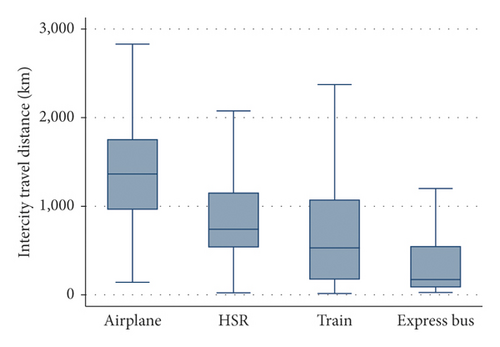
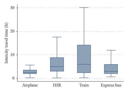
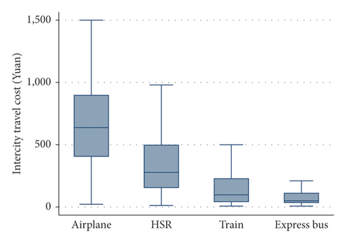
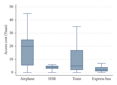
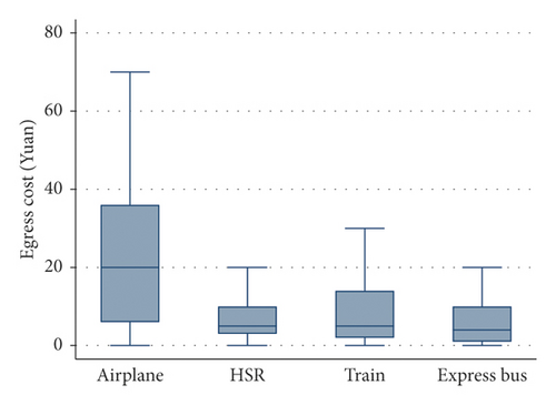
A total of 985 valid questionnaires were used in this study after denoising and cleaning. Among the records, 161 (16.3%) were for air travel, 369 (37.5%) for HSR, 299 (30.4%) for train, and 156 (15.8%) for express bus. In addition to the survey responses, the travel distance was calculated by Baidu Maps [48] using the real route between the origin and destination cities. The intercity travel time was measured based on the schedule corresponding to the vehicle number and the origin and destination cities [47]. Table 2 presents descriptions and frequencies of category variables for four travel modes. Figure 1 intuitively describes the continuous variables for different modes by box plots.

Table 2. Descriptions of category variables.

Variable	Description	Code	Frequency
Variable	Description	Code	Airplane	HSR	Train	Express bus	Total
Gender	Male	1	99	205	166	99	569
Gender	Female	0	62	164	133	57	416

Age	<19	1	1	10	7	5	23
	20–29	2	51	124	145	87	407
	30–39	3	61	135	90	33	319
	40–49	4	32	65	38	19	154
	50–59	5	13	30	16	6	65
	60 and above	6	3	5	3	6	17

Career	Enterprise personnel	1	47	78	71	17	213
	Government personnel	2	31	83	43	17	174
	Student	3	34	82	81	81	278
	Farmer	4	8	22	22	5	57
	Self-employed	5	26	51	48	18	143
	Others	6	15	53	34	18	120

Monthly income	<3K yuan	1	33	81	108	86	213
	3-4K yuan	2	22	103	45	18	174
	4-5K yuan	3	48	122	57	27	278
	5-6K yuan	4	38	40	46	17	57
	6-7K yuan	5	7	10	16	0	143
	>7K yuan	6	13	13	27	8	120

Car ownership	Yes	0	93	176	144	40	453
Car ownership	No	1	68	193	155	116	532

Travel purpose	Mandatory	1	86	156	155	77	474
Travel purpose	Leisure	0	75	213	144	79	511

Ticket purchasing method	Online	1	159	324	213	92	788
Ticket purchasing method	Counter	0	2	45	86	64	197

Access mode	Public transit	1	94	263	197	123	677
Access mode	Private car or taxi	0	67	106	102	33	308

Access time	0–0.5 h	1	28	106	105	79	318
	0.5–1 h	2	51	169	98	45	363
	1–1.5 h	3	82	94	96	32	304

Safety	Very unsafe	1	0	0	0	0	0
	Unsafe	2	1	0	3	6	10
	General	3	19	33	74	49	175
	Safe	4	78	173	167	77	495
	Very safe	5	63	163	55	24	305

Comfort	Very uncomfortable	1	0	0	1	7	8
	Uncomfortable	2	4	4	19	25	52
	General	3	23	57	109	56	245
	Comfortable	4	90	221	145	60	516
	Very comfortable	5	44	87	25	8	164

Punctuality	Very unpunctual	1	0	0	0	0	0
	Unpunctual	2	7	6	13	13	39
	General	3	53	57	80	61	251
	Punctual	4	85	199	166	75	525
	Very punctual	5	16	107	40	7	170

Egress mode	Public transit	1	94	297	214	108	713
Egress mode	Private car or taxi	0	67	72	85	48	272

Egress time	0–0.5 h	1	31	179	169	110	489
	0.5–1 h	2	73	119	100	30	322
	1–1.5 h	3	57	71	30	15	173

Details are in the caption following the image — **Figure 1 (a)**
Open in figure viewer PowerPoint

Description of continuous variables. (a) Intercity travel distance. (b) Intercity travel time. (c) Intercity travel cost. (d) Access cost. (e) Egress cost.

4. Methodology

4.1. Mixed Multinomial Logit Model

Compared with the traditional multinomial logit model, the mixed multinomial logit model allows all parameters to vary randomly across observations Mannering et al., 2016; Seraneeprakarn et al., 2017; [17, 23]. In this way, more data features can be extracted to improve the accuracy of regression [17]. The mixed multinomial logit model is described as

(1)

where Z_ji represents the choice of travel mode i by the j^th passenger, X = [x_i1, x_i2, …, x_iK] is a 1 × K vector of independent variables, and

is a coefficient vector.

In this study, the random parameters in the mixed multinomial logit model are assumed to be normally distributed as β ~ N(υ, Ψ), with

and

. Specifically,

(2)

The likelihood function of the model is

(3)

where N is the number of samples, I is the number of transportation modes, and ρ_ji is equal to 1 if the outcome for passenger j is i and is 0 otherwise [3, 27].

4.2. Full Bayesian Estimation

The posterior distribution of parameters is estimated by the full Bayesian inference on the base of the Markov chain Monte Carlo (MCMC) (Mannering et al., 2016; [27] In the full Bayesian approach, prior information and observed data are combined to obtain the parameters’ posterior distributions. The parameters of Ω can be represented as

(4)

The posterior distribution of parameters Ω according to Bayesian inference can be estimated as

(5)

where f(Ω|Z) is the posterior distribution of parameters Ω conditional on Z, f(Z, Ω) is the joint probability distribution of data set Z and parameters Ω, π(Ω) is the prior distribution of parameters Ω, and f(Z|Ω) is the likelihood conditional function based on parameters Ω (Mannering et al., 2016; [42]. Because of the lack of information, noninformative prior distributions for the random parameters in the model are adopted and expressed as follows:

(6)

(7)

where the mean of the random parameters follows the normal distribution, and the variance follows an inverse gamma distribution. Based on previous studies (Mannering et al., 2016; [46]), the parameters with overlines in equations (6) and (7) are hyperparameters,

(8)

Based on the prior distributions of parameters Ω, the posterior distribution f(Ω|Z) can be derived as follows:

(9)

4.3. Odds Ratio

The impact of significant factors can be assessed using the odds ratio (OR) [49, 50]. The OR of an explanatory variable represents the increment in the odds of the outcome if the value of the variable increases by one unit [50], which is calculated as

(10)

5. Results and Discussion

5.1. Modeling Results

To avoid correlation between intercity travel cost and time and travel distance, the intercity travel cost and time per hundred kilometers were calculated so as to standardize them [3, 12]. Multicollinearity testing and correlation analysis between each pair of variables were conducted to reduce estimation bias [47]. We used trains as the reference category, and the significant factors on intercity mode choice were identified using the Bayesian multinomial logit model and Bayesian mixed logit model, and Tables 3 and 4 show their respective parameter estimates. Significant variables at a 95% confidence level are retained in the tables. It is found that significant variables vary across modes. For example, age is significantly associated with airplanes and HSR choice, but not with the express bus.

Table 3. Parameter estimation from Bayesian multinomial logit model.

Variable	Airplane					HSR					Express bus
Variable	Mean	S.D.	2.5%	97.5%	OR	Mean	S.D.	2.5%	97.5%	OR	Mean	S.D.	2.5%	97.5%	OR
Age	—	—	—	—	—	0.2320	0.0898	0.0525	0.4098	1.2611	—	—	—	—	—
Car ownership (yes vs. no)	0.7630	0.2790	0.2228	1.3187	2.1446	0.3019	0.1285	0.0524	0.5431	1.3525	1.0466	0.1089	0.8547	1.2607	2.8479
Ticketing method (online vs. counter)	3.8221	0.4435	2.9720	4.6887	45.7020	0.6876	0.2334	0.2319	1.1427	1.9890	—	—	—	—	—
Travel purpose (mandatory vs leisure)	0.4430	0.2038	0.0731	0.8601	1.5573	—	—	—	—	—	—	—	—	—	—
Travel distance	0.0021	0.0004	0.0014	0.0028	1.0021	—	—	—	—	—	−0.0018	0.0003	−0.0023	−0.0012	0.9982
Standardized intercity travel cost	0.0874	0.2033	8.3459	9.1509	1.0913	0.0408	0.1015	3.8786	4.2649	1.0416	—	—	—	—	—
Standardized intercity travel time	−8.7058	0.3819	−8.7133	−8.6984	0.0002	−1.6856	0.1578	−1.6888	−1.6825	0.1853	0.0176	0.1955	0.0136	0.0213	1.0177
Safety	—	—	—	—	—	0.4788	0.1322	0.2014	0.7292	1.6142	—	—	—	—	—
Comfort	0.5972	0.1817	0.2400	0.9401	1.8171	0.4784	0.1078	0.2770	0.7035	1.6134	−0.4663	0.1119	−0.6844	−0.2479	0.6273
Punctuality	—	—	—	—	—	0.3557	0.1007	0.1614	0.5563	1.4271	−0.5674	0.1266	−0.8112	−0.3332	0.5670
Access time	0.4424	0.1920	0.0608	0.8085	1.5565	—	—	—	—	—	−0.4890	0.1211	−0.7285	−0.2553	0.6132
Egress time	0.8259	0.2038	0.4359	1.2334	2.2839	—	—	—	—	—	—	—	—	—	—
Intercept	−12.3802	0.3728	−13.0941	−11.6221	—	−6.4588	0.0867	−6.6117	−6.2834	—	4.4313	0.1747	4.1208	4.8361	—
DIC	1265.86

Table 4. Parameter estimation from Bayesian mixed multinomial logit model.

Variable	Airplane					HSR					Express bus
Variable	Mean	S.D.	2.50%	97.50%	OR	Mean	S.D.	2.50%	97.50%	OR	Mean	S.D.	2.50%	97.50%	OR
Age	0.3070	0.1304	0.0464	0.5684	1.3593	0.2048	0.0740	0.0612	0.3474	1.2272
Car ownership (yes vs. no)	0.9020	0.2431	0.4584	1.3964	2.4646	0.3579	0.0398	0.2802	0.4325	1.4304	0.9101	0.1385	0.6224	1.1830	2.4845
Ticket purchasing method (online vs. Counter)	1.3875	0.6436	0.1475	2.7089	4.0047	0.7536	0.1725	0.4197	1.0904	2.1245
Std. dev. of parameter distribution	0.8358	1.5022	0.0079	6.2454
Travel purpose (mandatory vs leisure)	1.0889	0.3387	0.4473	1.7911	2.9710
Travel distance	0.0021	0.0004	0.0014	0.0027	1.0021						−0.0018	0.0003	−0.0023	−0.0011	0.9982
Standardized intercity travel cost	0.0884	0.0072	0.0750	0.1030	1.0924	0.0434	0.0053	0.0333	0.0541	1.0443
Standardized intercity travel time	−8.9863	0.4566	−9.8979	−8.1441	0.0001	−1.7690	0.1050	−1.9738	−1.5488	0.1705
Safety						0.5185	0.0667	0.3960	0.6459	1.6794
Comfort	0.5129	0.1139	0.2967	0.7388	1.6702	0.8495	0.3396	0.2216	1.4898	2.3386	−0.4259	0.1230	−0.6948	−0.2041	0.6532
Std. dev. of parameter distribution						0.6738	0.9980	0.0079	3.5664						1.0000
Punctuality	−0.3233	0.1851	−0.6802	0.0520	0.7238	0.5702	0.2443	0.1034	1.0050	1.7687	−0.5349	0.1304	−0.7745	−0.2819	0.5857
Std. dev. of parameter distribution						0.3077	0.4813	0.0067	1.8824
Access time	0.3977	0.1498	0.1160	0.7023	1.4884						−0.3944	0.2017	−0.8375	−0.0453	0.6741
Std. dev. of parameter distribution											0.3375	0.5111	0.0071	1.8689
Egress time	0.8065	0.1656	0.4060	1.0077	2.2401						−0.1981	0.0611	−0.3203	−0.0748	0.8203
Intercept	−11.1867	0.2189	−11.6199	−10.7533	0.0000	−6.0312	0.2060	−6.4523	−5.6564	0.0024	4.0469	0.1027	3.8521	4.2625	57.2187
DIC	1240.95

The performance of these two regressions was compared using deviance information criterion (DIC), which was 1240.95 for the Bayesian mixed logit model and 1265.86 for the Bayesian multinomial logit model, indicating that the Bayesian mixed logit model performs better [51].

5.2. Interpretation of Model

The result from the Bayesian mixed logit model was selected for model interpretation due to its better performance. As shown in Table 4, age is found to affect passengers′ airplane and HSR choices versus train. The OR of age indicated that the odds of passengers taking an airplane or HSR instead of train increased by 35.93% and 22.72%, respectively, for every additional 10 years of age, perhaps because older passengers prefer comfortable and reliable transportation. However, age does not affect express bus choice compared to train, which is inconsistent with a previous study [12] that found that the 31–45 age group preferred train to coach. Car ownership is found to be significantly related to passengers’ choices of airplanes, trains, and express buses. The OR shows that passengers with cars were 2.4646, 1.4304, and 2.4845 times more likely to travel by airplane, HSR, and express bus, respectively, than passengers without cars. This intuitively suggests that passengers with cars are better able financially to choose safe and comfortable trips.

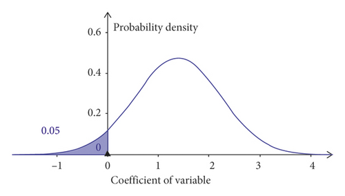
The ticket purchasing method has a significant relationship with the choice of airplane and HSR. The OR indicates that passengers who bought tickets online were 4.0047 and 2.1245 times more likely to travel by air and HSR, respectively, than those buying at the counter. It is straightforward that online ticketing is more convenient than other approaches in saving time for passengers. As shown in Figure 2, the normal distribution of the parameter is (1.3875, 0.8358) in association with airplane choice, indicating that 95.15% of online ticketing passengers have a higher probability of choosing an airplane compared to train, whereas the remaining 4.85% of online ticketing passengers have a lower probability of traveling by airplane compared to train. This result implies heterogeneous effects across ticketing methods.

Travel purposes significantly affect airplane choice. The OR of 2.9710 regarding this factor indicates that mandatory travel increased by 1.9710 times the odds of passengers’ traveling by airplane compared with the leisure travel purpose. This may be because passengers with mandatory travel are inclined to select a relatively fast travel mode.

Travel distance is significantly related to passengers’ airplane and express bus choices. An increase of 1 km leads to an increase of 0.21% and decrease of 0.18% in the probability of passengers traveling by air and express, respectively. This is consistent with the increase of the probability of choosing to fly with increasing travel distances. Conversely, the express bus was associated with shorter distances.

The standardized intercity travel cost is associated with airplane and HSR choices. Every 0.01 yuan increase in travel cost per kilometer leads to a 9.24% increase in the probability of choosing an airplane and 5.17% and 4.43% decreases in the probabilities of choosing a train and express bus, respectively. This is similar to a past study [12] indicating that standardized intercity travel costs play an important role in the choice of intercity travel modes.

The standardized intercity travel time is also linked to passengers’ choices of airplanes and HSR. Every 0.01 hour/km addition to intercity travel time leads to 99.99% and 82.95% reductions of the probabilities of travel by airplane and HSR, respectively. This result is supported by the study of Can [12], showing that adjusting intercity travel time per unit mileage is an important means by which transportation enterprises can attract passengers.

Safety is significantly related to the choice of HSR. According to OR analysis, the odds of passengers choosing an HSR over a train increase by 67.94% for each additional unit of safety demand. This suggests that passengers who have greater safety demands are more likely to travel on HSR.

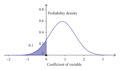
Based on the OR analysis, each incremental unit of comfort will cause 67.02%, 133.86%, and −34.68% increases in the odds of passengers choosing an airplane, HSR, and express bus, respectively. As can be expected, a cleaner and more comfortable service environment can be provided on airplanes and HSR, and the opposite holds on the express bus. The normal distribution (see Figure 3) of this parameter for HSR is (0.8495, 0.6738), indicating that 89.63% of passengers have a higher probability of choosing HSR with increasing demand for comfort, and the remaining 10.37% of passengers have a lower probability of choosing HSR compared to train with the increasing demand for comfort. This result implies heterogeneous effects across comfort.

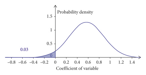
Punctuality is found to be significantly associated with passengers’ intercity travel mode choices. The results show that passengers with higher punctuality requirements tend to choose HSR. Each incremental unit of punctuality will cause 76.87%, −27.62%, and −41.43% increases in the odds of choosing HSR, airplane, and express bus, respectively. As shown in Figure 4, the normal distribution of the parameter for HSR is (0.5702, 0.3077), indicating that 96.81% of passengers have a higher probability of choosing HSR with increasing demands for punctuality, and the remaining 3.19% prefer the train with the increasing demand for punctuality.

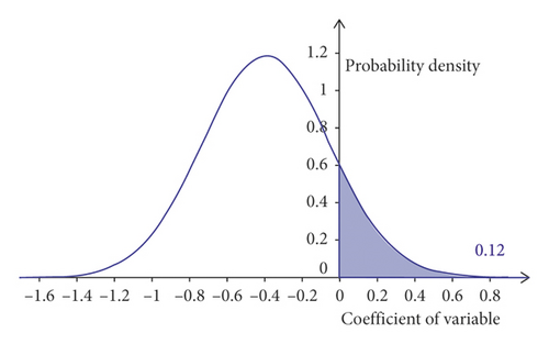
Access time is also found to be associated with airplane and express bus choices. Based on the OR analysis, each additional 30-minute increase in access time will cause 48.84% and −32.59% increases in the odds of choosing airplanes and express buses, respectively. As shown in Figure 5, the coefficient was normally distributed with (−0.3944, 0.3375) for the express bus, indicating that 87.87% of passengers who spend longer access time are less likely to choose express buses, while the remaining 12.13% of passengers spending longer access time are more likely to choose the express bus. The result confirms the heterogeneous effects across the access time. A similar finding can be found for the egress time. According to the OR, each additional 30 minutes of egress time will lead to 124.01% and −17.93% increases in odds of taking an airplane and express bus, respectively.

6. Conclusion

We explored the influence mechanism of competitive factors for intercity modes (i.e., airplane, HSR, train, and express bus) and found unobserved heterogeneity of significant factors in the intercity model choice. Passengers’ intercity travel activity data from Xi’an, China, were used for modeling. A mixed multinomial logit model was established to explore the relevant factors of intercity mode choice, which was compared with the Bayesian multinomial logit model. The proposed mixed multinomial logit model successfully captured the heterogeneous effects of some significant factors. It was found that the mixed multinomial logit model outperformed the Bayesian multinomial logit model according to the comparison of DIC. The results also showed that ticket purchasing method, comfort, punctuality, and access time had heterogeneous effects on intercity travel mode choice, appearing in the form of random parameters in the model.

These findings are helpful in providing relevant management strategies for intercity travel mode choices, are of significance for transportation development, and can provide information for decision-makers and planners. For decision-makers, the development of HSR is highly recommended because it has incomparable advantages such as punctuality, safety, and comfort. With the background of global aging, the elderly prefer HSR, which meets the needs of passengers for higher service quality. At the same time, improving the efficiency of HSR and common rail and adjusting their ticket prices are important means to promote the transfer of passengers from high-energy transport modes (such as airplane and express bus) to low-energy modes. For transportation planners, the layout of airports and railway stations, as well as connection modes, is an indivisible part of their competitiveness. For service providers, an efficient ticketing system has a significant impact on mode choice, particularly for express buses. There is an urgent need for an efficient online ticketing system. Finally, the model and its estimates can provide a reference for software companies to develop intelligent decision service systems for intercity travel mode choices.

The study has several limitations. We used data from only one city. Different cultural backgrounds and traffic environments could change travel mode choices. Therefore, data from other cities should be collected to verify the proposed model and findings. Such potential factors as temperature, humidity, rainfall, snowfall, and visibility were not explored. In the future, these factors can be incorporated into the model, and their impact on passengers’ intercity travel mode choices should be discussed. In addition, the comparison of the Bayesian mixed multinomial logit model with machine learning methods [52] is a valuable research field. Finally, although we found that some variables (e.g., ticket purchasing method, comfort, punctuality, and access time) have heterogeneous effects on passengers′ choices of intercity travel modes, their specific effects on traffic management still must be explored.

Conflicts of Interest

The authors declare no conflicts of interest.

Acknowledgments

This work was funded by the National Natural Science Foundation of China (no. 71701046), Shaanxi Natural Science Foundation Youth Project (no. 2017JQ5086), Shaanxi Education Department Special Science and Technology Project Science (no. 19JK0477), and Foundation Project of Xi’an University of Architectural Science and Technology (no. ZR18021 and QN1711).

Open Research

Data Availability

The data used to support the findings of this study are available from the corresponding author upon request.

References

1 Givoni M. and Dobruszkes F., A review of ex-post evidence for mode substitution and induced demand following the introduction of high-speed rail, Transport Reviews. (2013) 33, no. 6, 720–742, https://doi.org/10.1080/01441647.2013.853707, 2-s2.0-84889645321.
10.1080/01441647.2013.853707
Web of Science® Google Scholar
2 China National Railway Corporation, Database of National Bureau of Statistics of China, 2019, China National Railway Corporation, Beijing, China.
Google Scholar
3 Li X., Tang J., Hu X., and Wang W., Assessing intercity multimodal choice behavior in a touristy city: a factor analysis, Journal of Transport Geography. (2020) 86, https://doi.org/10.1016/j.jtrangeo.2020.102776.
10.1016/j.jtrangeo.2020.102776
PubMed Web of Science® Google Scholar
4 Zhang C.-X., Xu S., and Zhang J.-S., A novel variational Bayesian method for variable selection in logistic regression models, Computational Statistics & Data Analysis. (2019) 133, 1–19, https://doi.org/10.1016/j.csda.2018.08.025, 2-s2.0-85054553886.
10.1016/j.csda.2018.08.025
Web of Science® Google Scholar
5 Sun X., Zhang Y., and Wandelt S., Air transport versus high-speed rail: an overview and research agenda, Journal of Advanced Transportation. (2017) 2017, 18, 8426926, https://doi.org/10.1155/2017/8426926, 2-s2.0-85020033387.
10.1155/2017/8426926
Google Scholar
6 Xia W., Wang K., and Zhang A., Air Transport and High-Speed Rail Interactions in China: Review on Impacts of Low-Cost Carriers, Rail Speed, and Modal Integration, 2018, Emerald Publishing Ltd, Bingley, UK.
Google Scholar
7 Yang H., Burghouwt G., Wang J., Boonekamp T., and Dijst M., The implications of high-speed railways on air passenger flows in China, Applied Geography. (2018) 97, 1–9, https://doi.org/10.1016/j.apgeog.2018.05.006, 2-s2.0-85054309346.
10.1016/j.apgeog.2018.05.006
PubMed Web of Science® Google Scholar
8 Yang H., Zhang Q., and Wang Q., Airline deregulation, market competition, and impact of high-speed rail on airlines in China, Airline Economics in Asia. (2018) Emerald Publishing Ltd, Bingley, UK, https://doi.org/10.1108/s2212-160920180000007006, 2-s2.0-85064637035.
10.1108/S2212-160920180000007006
Google Scholar
9 Tang B., Li X., Yu B., and Wei Y., Sustainable development pathway for intercity passenger transport: a case study of China, Applied Energy. (2019) 254, https://doi.org/10.1016/j.apenergy.2019.113632, 2-s2.0-85071022667.
10.1016/j.apenergy.2019.113632
Web of Science® Google Scholar
10 Bhat C. R., Accommodating variations in responsiveness to level-of-service measures in travel mode choice modeling, Transportation Research Part A: Policy and Practice. (1998) 32, no. 7, 495–507, https://doi.org/10.1016/s0965-8564(98)00011-1, 2-s2.0-0031597048.
10.1016/S0965-8564(98)00011-1
Web of Science® Google Scholar
11 Wen C.-H., Wang W.-C., and Fu C., Latent class nested logit model for analyzing high-speed rail access mode choice, Transportation Research Part E: Logistics and Transportation Review. (2012) 48, no. 2, 545–554, https://doi.org/10.1016/j.tre.2011.09.002, 2-s2.0-83555178499.
10.1016/j.tre.2011.09.002
Web of Science® Google Scholar
12 Can V. V., Estimation of travel mode choice for domestic tourists to Nha Trang using the multinomial probit model, Transportation Research Part A: Policy and Practice. (2013) 49, 149–159, https://doi.org/10.1016/j.tra.2013.01.025, 2-s2.0-84873947355.
10.1016/j.tra.2013.01.025
Web of Science® Google Scholar
13 Miskeen M. A. A. B., Alhodairi A. M., and Rahmat R. A. A. B. O., Modeling a multinomial logit model of intercity travel mode choice behavior for all trips in Libya, International Journal of Civil and Environmental Engineering. (2013) 7, no. 9, 636–645.
Google Scholar
14 Román C., Martín J. C., Espino R., Cherchi E., Ortúzar J. d. D., Rizzi L. I., González R. M., and Amador F. J., Valuation of travel time savings for intercity travel: the Madrid-Barcelona corridor, Transport Policy. (2014) 36, 105–117, https://doi.org/10.1016/j.tranpol.2014.07.007, 2-s2.0-84907535384.
10.1016/j.tranpol.2014.07.007
Web of Science® Google Scholar
15 Li Z.-C. and Sheng D., Forecasting passenger travel demand for air and high-speed rail integration service: a case study of Beijing-Guangzhou corridor, China, Transportation Research Part A: Policy and Practice. (2016) 94, 397–410, https://doi.org/10.1016/j.tra.2016.10.002, 2-s2.0-84991730363.
10.1016/j.tra.2016.10.002
Web of Science® Google Scholar
16 Sperry B. R., Burris M., and Woosnam K. M., Investigating the impact of high-speed rail equipment visualization on mode choice models: case study in central Texas, Case Studies on Transport Policy. (2017) 5, 560–572, https://doi.org/10.1016/j.cstp.2017.10.004, 2-s2.0-85031501075.
10.1016/j.cstp.2017.10.004
Google Scholar
17 Guo Y., Sayed T., and Zaki M. H., Evaluating the safety impacts of powered two wheelers on a shared roadway in China using automated video analysis, Journal of Transportation Safety & Security. (2019) 11, no. 4, 414–429, https://doi.org/10.1080/19439962.2018.1447058, 2-s2.0-85043771258.
10.1080/19439962.2018.1447058
Web of Science® Google Scholar
18 Waseem M., Ahmed A., and Saeed T. U., Factors affecting motorcyclists’ injury severities: an empirical assessment using random parameters logit model with heterogeneity in means and variances, Accident Analysis & Prevention. (2019) 123, 12–19, https://doi.org/10.1016/j.aap.2018.10.022, 2-s2.0-85056468615.
10.1016/j.aap.2018.10.022
PubMed Web of Science® Google Scholar
19 Greene W. H., Hensher D. A., and Rose J., Accounting for heterogeneity in the variance of unobserved effects in mixed logit models, Transportation Research Part B: Methodological. (2006) 40, no. 1, 75–92, https://doi.org/10.1016/j.trb.2005.01.005, 2-s2.0-24344443637.
10.1016/j.trb.2005.01.005
Web of Science® Google Scholar
20 Behnood A. and Mannering F., The effect of passengers on driver-injury severities in single-vehicle crashes: a random parameters heterogeneity-in-means approach, Analytic Methods in Accident Research. (2017) 14, 41–53, https://doi.org/10.1016/j.amar.2017.04.001, 2-s2.0-85019206304.
10.1016/j.amar.2017.04.001
Web of Science® Google Scholar
21 Behnood A. and Mannering F., Determinants of bicyclist injury severities in bicycle-vehicle crashes: a random parameters approach with heterogeneity in means and variances, Analytic Methods in Accident Research. (2017) 16, 35–47, https://doi.org/10.1016/j.amar.2017.08.001, 2-s2.0-85027543181.
10.1016/j.amar.2017.08.001
Web of Science® Google Scholar
22 Huang H., Chang F., Zhou H., and Lee J., Modeling unobserved heterogeneity for zonal crash frequencies: a Bayesian multivariate random-parameters model with mixture components for spatially correlated data, Analytic Methods in Accident Research. (2019) 24, https://doi.org/10.1016/j.amar.2019.100105, 2-s2.0-85072708197.
10.1016/j.amar.2019.100105
Web of Science® Google Scholar
23 Hou Q., Huo X., Leng J., and Cheng Y., Examination of driver injury severity in freeway single-vehicle crashes using a mixed logit model with heterogeneity-in-means, Physica A: Statistical Mechanics and its Applications. (2019) 531, https://doi.org/10.1016/j.physa.2019.121760, 2-s2.0-85067053253.
10.1016/j.physa.2019.121760
Web of Science® Google Scholar
24 M Hamed M. and Al-Eideh B., An exploratory analysis of traffic accidents and vehicle ownership decisions using a random parameters logit model with heterogeneity in means, Analytic Methods in Accident Research. (2020) 25, https://doi.org/10.1016/j.amar.2020.100116.
10.1016/j.amar.2020.100116
Web of Science® Google Scholar
25 Rukhin A. L., Estimating heterogeneity variances to select a random effects model, Journal of Statistical Planning and Inference. (2019) 202, 1–13, https://doi.org/10.1016/j.jspi.2018.12.003, 2-s2.0-85061625533.
10.1016/j.jspi.2018.12.003
Web of Science® Google Scholar
26 Shahram H., Liping F., Lalita T., and Lawrence J., Benchmarking regions using a heteroskedastic grouped random parameters model with heterogeneity in mean and variance: applications to grade crossing safety analysis, Analytic Methods in Accident Research. (2018) 19, 33–48.
10.1016/j.amar.2018.06.003
Web of Science® Google Scholar
27 Guo Y., Sayed T., and Essa M., Real-time conflict-based Bayesian Tobit models for safety evaluation of signalized intersections, Accident; Analysis and prevention. (2020) 144, 105660–105711, https://doi.org/10.1016/j.aap.2020.105660.
10.1016/j.aap.2020.105660
PubMed Web of Science® Google Scholar
28 Alnawmasi N. and Mannering F., A statistical assessment of temporal instability in the factors determining motorcyclist injury severities, Analytic Methods in Accident Research. (2019) 22, 100090, https://doi.org/10.1016/j.amar.2019.100090, 2-s2.0-85064234017.
10.1016/j.amar.2019.100090
Web of Science® Google Scholar
29 Yu M., Zheng C., and Ma C., Analysis of injury severity of rear-end crashes in work zones: a random parameters approach with heterogeneity in means and variances, Analytic Methods in Accident Research. (2020) 27, 1–14, https://doi.org/10.1016/j.amar.2020.100126.
10.1016/j.amar.2020.100126
Web of Science® Google Scholar
30 Chen X., Li Z., Yang Y., Qi L., and Ke R., High-resolution vehicle trajectory extraction and denoising from aerial videos, IEEE Transactions on Intelligent Transportation Systems. (2021) 22, no. 5, 3190–3202, https://doi.org/10.1109/tits.2020.3003782.
10.1109/TITS.2020.3003782
Web of Science® Google Scholar
31 Hess S., Spitz G., Bradley M., and Coogan M., Analysis of mode choice for intercity travel: application of a hybrid choice model to two distinct US corridors, Transportation Research Part A: Policy and Practice. (2018) 116, 547–567, https://doi.org/10.1016/j.tra.2018.05.019, 2-s2.0-85050149122.
10.1016/j.tra.2018.05.019
Web of Science® Google Scholar
32 Forinash C. V. and Koppelman F. S., Application and interpretation of nested logit models of intercity mode choice, Transportation Research Record Journal of the Transportation Research Board. (1993) 1413, 98–106.
Google Scholar
33 Bhat C. R., An endogenous segmentation mode choice model with an application to intercity travel, Transportation Science. (1997) 31, no. 1, 34–48, https://doi.org/10.1287/trsc.31.1.34, 2-s2.0-0031070052.
10.1287/trsc.31.1.34
Web of Science® Google Scholar
34 Martín J. C., Román C., García-Palomares J. C., and Gutiérrez J., Spatial analysis of the competitiveness of the high-speed train and air transport: the role of access to terminals in the Madrid-Barcelona corridor, Transportation Research Part A: Policy and Practice. (2014) 69, 392–408, https://doi.org/10.1016/j.tra.2014.09.010, 2-s2.0-84907951183.
10.1016/j.tra.2014.09.010
Web of Science® Google Scholar
35 Zheng Z., Washington S., Hyland P., Sloan K., and Liu Y., Preference heterogeneity in mode choice based on a nationwide survey with a focus on urban rail, Transportation Research Part A: Policy and Practice. (2016) 91, 178–194, https://doi.org/10.1016/j.tra.2016.06.032, 2-s2.0-84978253775.
10.1016/j.tra.2016.06.032
Web of Science® Google Scholar
36 Bhat C. R., A heteroscedastic extreme value model of intercity travel mode choice, Transportation Research Part B: Methodological. (1995) 29, no. 6, 471–483, https://doi.org/10.1016/0191-2615(95)00015-6, 2-s2.0-0029473530.
10.1016/0191-2615(95)00015-6
Web of Science® Google Scholar
37 Wang Y., Li L., Wang L., Moore A., Staley S., and Li Z., Modeling traveler mode choice behavior of a new high-speed rail corridor in China, Transportation Planning and Technology. (2014) 37, no. 5, 466–483, https://doi.org/10.1080/03081060.2014.912420, 2-s2.0-84901454007.
10.1080/03081060.2014.912420
Web of Science® Google Scholar
38 Ashiabor S., Baik H., and Trani A., Logit models for forecasting nationwide intercity travel demand in the United States, Transportation Research Record: Journal of the Transportation Research Board. (2007) 2007, no. 1, 1–12, https://doi.org/10.3141/2007-01, 2-s2.0-38849167432.
10.3141/2007-01
Google Scholar
39 Lee J.-H., Chon K.-S., and Park C., Accommodating heterogeneity and heteroscedasticity in intercity travel mode choice model: formulation and application to HoNam, South Korea, high-speed rail demand analysis, Transportation Research Record: Journal of the Transportation Research Board. (2004) 1898, no. 1, 69–78, https://doi.org/10.3141/1898-09, 2-s2.0-19944403244.
10.3141/1898-09
Google Scholar
40 Srinivasan S., Bhat C. R., and Holguin-Veras J., Empirical analysis of the impact of security perception on intercity mode choice, Transportation Research Record: Journal of the Transportation Research Board. (2006) 1942, no. 1, 9–15, https://doi.org/10.1177/0361198106194200102.
10.1177/0361198106194200102
Google Scholar
41 Li X., Wang W., Xu C., Li Z., and Wang B., Multi-objective optimization of urban bus network using cumulative prospect theory, Journal of Systems Science and Complexity. (2015) 28, no. 3, 661–678, https://doi.org/10.1007/s11424-015-2049-0, 2-s2.0-84928888453.
10.1007/s11424-015-2049-0
Web of Science® Google Scholar
42 Li H., Wang K., Yu K., and Zhang A., Are conventional train passengers underserved after entry of high-speed rail?-evidence from Chinese intercity markets, Transport Policy. (2020) 95, 1–9, https://doi.org/10.1016/j.tranpol.2020.05.017.
10.1016/j.tranpol.2020.05.017
CAS Web of Science® Google Scholar
43 Guo Y., Li Z., Wu Y., and Xu C., Exploring unobserved heterogeneity in bicyclists’ red-light running behaviors at different crossing facilities, Accident Analysis & Prevention. (2018) 115, 118–127, https://doi.org/10.1016/j.aap.2018.03.006, 2-s2.0-85043754624.
10.1016/j.aap.2018.03.006
PubMed Web of Science® Google Scholar
44 Zhang A., Wan Y., and Yang H., Impacts of high-speed rail on airlines, airports and regional economies: a survey of recent research, Transport Policy. (2019) 81, 1–19, https://doi.org/10.1016/j.tranpol.2019.06.010, 2-s2.0-85067938288.
10.1016/j.tranpol.2019.06.010
Web of Science® Google Scholar
45 Afghari A. P., Haque M. M., Washington S., and Smyth T., Effects of globally obtained informative priors on Bayesian safety performance functions developed for Australian crash data, Accident Analysis & Prevention. (2019) 129, 55–65, https://doi.org/10.1016/j.aap.2019.04.023, 2-s2.0-85065702911.
10.1016/j.aap.2019.04.023
PubMed Web of Science® Google Scholar
46 Guo Y., Sayed T., Zheng L., and Essa M., An extreme value theory based approach for calibration of microsimulation models for safety analysis, Simulation Modelling Practice and Theory. (2021) 106, 1–16, https://doi.org/10.1016/j.simpat.2020.102172.
10.1016/j.simpat.2020.102172
Web of Science® Google Scholar
47 Li X., Ma R., Guo Y., Wang W., Yan B., and Chen J., Investigation of factors and their dynamic effects on intercity travel modes competition, Travel Behaviour and Society. (2021) 23, 166–176, https://doi.org/10.1016/j.tbs.2021.01.003.
10.1016/j.tbs.2021.01.003
Web of Science® Google Scholar
48 Baidu Company, Baidu Map, 2018, https://map.baidu.com.
Google Scholar
49 Washington S., Karlaftis M., and Mannering F., Statistical and Econometric Methods for Transportation Data Analysis, 2010, 2nd edition, Taylor & Francis Group, Boca Raton, FL, USA, 200–230.
Google Scholar
50 Li X., Fan J., Wu Y., Chen J., and Deng X., Exploring influencing factors of passenger satisfaction toward bus transit in small-medium city in China, Discrete Dynamics in Nature and Society. (2020) 2020, 11, 8872115, https://doi.org/10.1155/2020/8872115.
10.1155/2020/8872115
Web of Science® Google Scholar
51 Chen E. and Tarko A. P., Modeling safety of highway work zones with random parameters and random effects models, Analytic Methods in Accident Research. (2014) 1, 86–95, https://doi.org/10.1016/j.amar.2013.10.003, 2-s2.0-84893518643.
10.1016/j.amar.2013.10.003
Google Scholar
52 Chen X., Lu J., Zhao J., Qu Z., Yang Y., and Xian J., Traffic flow prediction at varied time scales via ensemble empirical mode decomposition and artificial neural network, Sustainability. (2020) 12, no. 9, https://doi.org/10.3390/su12093678.
10.3390/su12093678
Web of Science® Google Scholar

Citing Literature

All articles

Exploring Influencing Factors of Intercity Mode Choice from View of Entire Travel Chain

Abstract

1. Introduction

2. Literature Review