Hard Disk Drive Failure Prediction for Mobile Edge Computing Based on an LSTM Recurrent Neural Network
Abstract
With the increase in intelligence applications and services, like real-time video surveillance systems, mobile edge computing, and Internet of things (IoT), technology is greatly involved in our daily life. However, the reliability of these systems cannot be always guaranteed due to the hard disk drive (HDD) failures of edge nodes. Specifically, a lot of read/write operations and hazard edge environments make the maintenance work even harder. HDD failure prediction is one of the scalable and low-overhead proactive fault tolerant approaches to improve device reliability. In this paper, we propose an LSTM recurrent neural network-based HDD failure prediction model, which leverages the long temporal dependence feature of the drive health data to improve prediction efficiency. In addition, we design a new health degree evaluation method, which stores current health details and deterioration. The comprehensive experiments on two real-world hard drive datasets demonstrate that the proposed approach achieves a good prediction accuracy with low overhead.
1. Introduction
The applications and services are greatly increasing recently, and global spending on the IoT reached 1.29 trillion dollars in 2020. For example, video surveillance is widely used in public and private security environments, accompanied with the popularity of outdoor cameras, the cost of data storage, and transmission is enormous [1]. To guarantee the performance of the surveillance systems, mobile edge computing solutions and IoT technologies are applied to process and transfer huge amounts of data in real-time [2]. The edge node is responsible for collecting data from one or more sensors and performing lightweight preprocessing computations. Thus, frequent read and write operations, combined with hazard edge environments (such as violent vibration and high temperatures) lead to high HDD failure rates. It greatly influences the reliability and performance of surveillance systems.
Passive failure tolerance is a common technique used to improve storage system reliability in data centers [3]. However, this technique does not work well in the mobile edge computing environment due to the high cost and poor scalability [4]. Therefore, it is very urgent to develop suitable proactive failure tolerance approaches.
The HDD failure prediction method usually analyzes drive health data and replacement logs to build a classification model; then, it will indicate the soon-to-fail HDDs. Once an impending failure is detected, the prediction system alerts the administrator to backup data and to replace drives. HDD manufacturers usually adopt threshold algorithms, which are built based on SMART (Self-Monitoring Analysis and Reporting Technology) data [5]. Unfortunately, the failure detection rate (FDR) of this method is very low, at only 3–10%, and the false alarm rate (FAR) is approximately 0.1% [5]. The low accuracy of failure prediction hinders the effectiveness of proactive fault tolerant approaches.
To improve the performance of HDD failures prediction, many machine-learning-based prediction approaches have been proposed, including Bayesian algorithms [6–9], support vector machine (SVM) [10], classification tree (CT) [11, 12], random forest (RF) [13, 14], artificial neural network (ANN) [15], convolution neural network (CNN) [16], and recurrent neural network (RNN) [17, 18]. RNN-based prediction models achieve the highest FDRs, and RF-based models attain the lowest FARs. The reason is that the temporal dependence of drive health data is extracted by RNN models to acquire the characteristics of drive deterioration, while early researchers [5, 7] seldom utilize the time sequence feature since the dataset scale is small. However, traditional RNN models only keep short-term memory due to the gradient vanishing or exploding [19]. To address this issue, some researchers [17, 19] adopted a segmentation method to simplify drive deterioration. Unfortunately, comparing with cloud computing, the worse environmental conditions in mobile edge computing lead to more complicated drive deterioration. Hence, the method does not work well. In addition, labeling accuracy of HDD health status is also one of the major determinant factors for prediction performance. Binary methods and deterioration degrees are widely used approaches, but the former neglects the deterioration process of HDDs which is highly related to current health status, and the latter only takes time sequence into consideration. Sample imbalance is also a major hindrance for HDD failure prediction as the number of good drives is far more than the failed drives in the training dataset.
In this paper, we apply the long short-term memory (LSTM) RNN to detect abnormal drive health samples according to the long temporal dependence feature of drive health data. LSTM models complex multivariate sequences accurately. To improve the accuracy of training sample labeling, we propose a novel health degree evaluation approach which simultaneously considers both the time-sequence features and the drive health status to comprehensively depict the deterioration of drives. To address the issue of imbalanced samples, we use a k-means clustering-based undersampling method to reduce the sample scale of good drives in the training set. It retains the characteristics of good drive samples and dramatically lowers the computation overhead.
- (1)
We propose an LSTM-RNN-based HDD failure prediction model for mobile edge computing environment. It extracts the long-term temporal dependence feature of drive health data to improve the accuracy of health degree computation.
- (2)
A health degree evaluation method is presented, which takes into account the time-series features and current health status of drives to solve the labeling issue in the training set.
- (3)
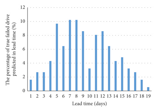
We performed a comprehensive evaluation with two real-world datasets from production data centers. The experimental results show that the proposed prediction model can archive an FDR of 94.49% with an FAR of 0.09%, and the lead times of most drives are less than 168 hours. The majority of soon-to-fail drives are predicted within 7 days, which is reasonable and acceptable.
The remainder of this paper is structured as follows. Section 2 reviews the background information of SMART, evaluation of drive health and related works. Section 3 introduces the LSTM-RNN-based prediction model and the HDD health degree evaluation method. Section 4 presents the experimental results, including a comparison with the state-of-the-art failure prediction approaches. Section 5 concludes the paper.
2. Background and Related Work
2.1. SMART
SMART is a self-monitoring system used to collect and report various performance indicators of HDDs, which is supported by almost all HDD manufactures [5]. SMART allows up to 30 internal drive attributes such as reallocated sector count (RSC), spin up time (SUT), and seek error rate (SER). Every attribute has five fields, raw data, value, threshold, worst value, and status. The raw data are the values measured by a sensor or a counter. The value is the normalized value of the current raw data; the algorithm for computing the values is defined by HDD manufacturers and is distinct between manufacturers. SMART issues a failure alarm to the user when the value of any attribute exceeds the given threshold at which it becomes a warning.
The SMART drive attributes can be roughly categorized into two groups, incremental counting and cumulative counting [20]. The former records incremental error counts over a fixed time interval. Most of the SMART attributes belong to this group, such as SUT, which is the period of time from power on to a readiness for data transfer. RSC is the count of reallocated sectors, which is an indicator of the health status of the disk media; this attribute belongs to the cumulative counting group. For cumulative counting attributes, their values and change rates correlate strongly with degradation of the drives and are helpful for detecting abnormal SMART samples. Hence, we add the value as well as the change rates of SMART attributes to the candidate feature subset.
2.2. Evaluation of Drive Health
Drive health evaluation influences the prediction accuracy of soon-to-fail drives directly and primarily falls into three groups: the binary method [8, 20], phase method [17], and health degree method [11, 18, 21].
The binary method categorizes drive health into two states: failed and good. The drive deterioration is usually a gradual process; however, these evaluation methods neglected the change process of drive health, which leads to unsatisfactory FDRs and a large range in lead times.
The phase method separates the process of drive degradation into several phases. Xu et al. [17] classified the health status of the drive into six levels that gradually decrease over time. Levels 6 and 5 indicate that the drive is good and fair, respectively. Levels 1–4 mean that the drive is going to fail. Level 1 indicates that the remaining time is less than 72 hours. The standard of interval division in this method depends on experience.
The health degree method builds functions to describe drive degradation. Zhu et al. [10] used a linear function to describe the relation between deterioration and time sequence, where the value range of this function is [−1, 0]. However, the health degree of these evaluation functions only changes with time, and the drive health also changes as the system workload fluctuates in a real-world storage systems. Therefore, linear evaluation methods also cannot describe the deterioration process accurately enough. Huang et al. [21] proposed a quantization method for evaluating the health state of HDDs based on Euclidean distance methods and divided the failed drives into three groups by analyzing the last drive health samples. A CART-based prediction model was built for each group of drives. The researchers assumed that the drives in a group have a similar deterioration process and built deterioration models for each group. The drive has complex structure, and the drive deterioration is affected by inner and outer factors, such as health status, workload, and age. Health degree calculated simply based on Euclidean distances involves nonignored noises. Therefore, the evaluation method in our proposed model takes account of current drive health status and deterioration together to improve the accuracy of sample labeling.
2.3. Prediction of Soon-To-Fail HDDs
Prediction of soon-to-fail HDDs usually employs statistical approaches, Bayesian approaches, SVM, BPNN, decision tree, random forest, RNN, and CNN.
Considering that many SMART attributes are nonparametrically distributed, Hughes et al. [20] adopted a multivariate rank-sum test and an OR-ed single variate test to detect soon-to-fail drives. The rank-sum test is only used in feature selection for later related research [22].
The Bayesian approach is commonly used in failure detection. Ma et al. [9] found that RSC correlates with drive failure and proposed RAIDShield, which uses Bayes to predict drive failures on RAID storage systems. This approach eliminated 88% of triple disk errors. The Bayesian network failure prediction method has been used with transfer learning so that HDD models with an abundance of data can be used to build prediction models for drives with a lack of data [6]. The Bayesian network-based method for failure prediction in HDDs (BNFH) [7] was proposed to estimate the remaining life of HDDs.
A BPNN-based model and an improved SVM model [10] were developed on a SMART dataset from the data center of Baidu Inc. The BPNN model achieved a higher FDR than SVM, and SVM obtained a lower FAR. The experimental data contained 22,962 good drives and 433 failed drives, and the scale of this dataset is much larger than the datasets in previous studies.
Li et al. [11] proposed CT-based and classification and regression tree (CART)-based prediction models that achieved an FDR of 95% and an FAR of 0.1%. The good prediction performance is due to the health degree model they proposed and a bigger experimental dataset. Rincón et al. [23] used a decision tree to predict hard disk failures owing to missing SMART values [24]. Kaur and Kaur [12] introduced a voting-based decision tree classifier to predict HDD failures and an R-CNN-based approach for health status estimation. A prediction model using online random forests (ORFs), which evolve as new HDDs health data arrived, was proposed to achieve online failures prediction for HDD [13]. A part-voting RF-based failure prediction for drives was proposed to differentiate failure prediction [14].
Deep neural networks achieve better performance than the others. A temporal CNN-based model for system-level hardware failure prediction was proposed to extract the discrete time-series data [16]. An RNN-based model was used for health status assessment and failure prediction for HDDs [17]. A layer-wise perturbation-based adversarial training for hard drive health degree prediction was also proposed [18]. These networks have also become popular in mobile edge computing [24, 25].
The works described above achieve good prediction efficiency; however, there is still much room for improvement. In this paper, we attempt to use an LSTM RNN for soon-to-fail HDD prediction to extract long temporal dependence feature of drive health data and propose a new health degree evaluation.
3. The Proposed Method
In this section, we start with an introduction to an LSTM-RNN-based prediction model in Subsection 3.1 and then present the health degree evaluation method in Subsection 3.2.
3.1. LSTM-RNN-Based Prediction Model
RNNs have been extensively used for various applications, such as language understanding [26], image processing [27], and computer vision [28]. Unlike ANNs, RNNs use their internal memories to process arbitrary sequences of input samples. Therefore, RNNs are chosen to extract temporal dependence feature of drive health data in our prediction model to calculate the health degree of drives.
Through use of an RNN, the historical drive health data are persistently transmitted and the time sequence of drive health data can be used. However, it is difficult for RNNs to learn long-range dependence because of gradient vanishing or exploding [29, 30]. The former describes the exponential decrease in the gradient for long-term cells to zero, and the latter describes the opposite event. To address these issues, an LSTM architecture was proposed [19, 31], which has become popular for many applications [32, 33]. During the drive deterioration process, certain health status changes and workloads influence HDD health over a long period; LSTM can account for these long sequences. Hence, we build a drive failure prediction model based on LSTM networks to take advantage of the temporal dependence feature of drive health data.
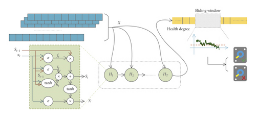
The value of sigmoid is between “0” and “1,” where “0” means completely forgotten and “1” means completely recorded.
3.2. Health Degree Evaluation Method for HDD
The quality of the training dataset, such as sample labeling and noises, determines the performance of the prediction model when using deep learning. HDD deterioration is a gradual process; we adopt health degree rather than a binary method to label drive health samples as a way to record the change of drive health. Health change trends and rates are influenced by usage and the current health status of the drive, so we take health status as well as deterioration into account to evaluate HDD health degree.
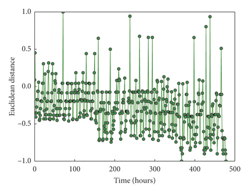
Figure 2 describes the health degree of a drive based on similarity. It is obvious that there are large random fluctuations, and the health degree at some time is very close to −1 when they still have more than 100 hours before failure. Nevertheless, according to the HDD degradation process, the health degree of a sample approaches −1 as it approaches the end of its life. Therefore, transform functions are adopted to reinforce the health status trends. We introduce an exponential function or a logarithmic function as the transformation function. More specifically, we import the similarity into the transform function and regard the function result as the health degree of drive at a given time. Algorithm 1 details the process of calculating health degree for a failed HDD in the training set.
-
Algorithm 1: The algorithm for calculating the health degree of a soon-to-fail HDD.
-
Input:
-
(1) Health samples of a drive: healthsamples
-
(2) The number of sample features: featuresNum
-
(3) Transformation function: f(⋅)
-
(4) Weights of health status and time: ω1, ω2
-
Output:
-
Health degree of a drive: drive_health_degree
-
Begin
-
(1) last = healthsamples [len (healthsamples) – 1]
-
(2) for sample in healthsamples
-
(3) while i < featuresNum
-
(4) o ⟵ o + pow (sample [i] – last[i], 2.0)
-
(5) i ⟵ i + 1
-
(6) Endwhile
-
(7) O. append (sqrt (o))
-
(8) endfor
-
//Standardizing the values of O to [−1, 1]
-
(9) O ⟵ standard (O)
-
(10) while i < len (healthsamples)
-
(11) E[i] ⟵ f(i)
-
(12) i ⟵ i + 1
-
(13) Endwhile
-
(14) E ⟵ standard (E)
-
(15) while i < len(healthsamples)
-
(16) health_degree [i] ⟵ ω1O[i] + ω2E[i]
-
(17) Endwhile
-
(18) return health_degree
-
End
Our evaluation method reinforces the decreasing trend in health degree along with time and retains the drive health status details based on similarity. Figure 3 shows the result of the health degree evaluation method for a failed HDD. The red line is computed by a logarithmic function, and the blue line is computed by an exponential function. We prefer the exponential function because the trend of the blue line’s decline is more obvious at the end of the period before HDD failure.
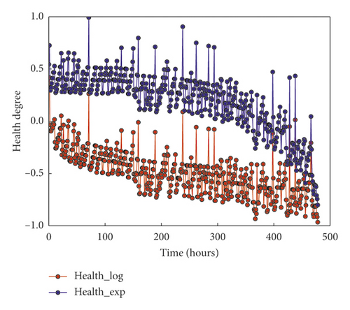
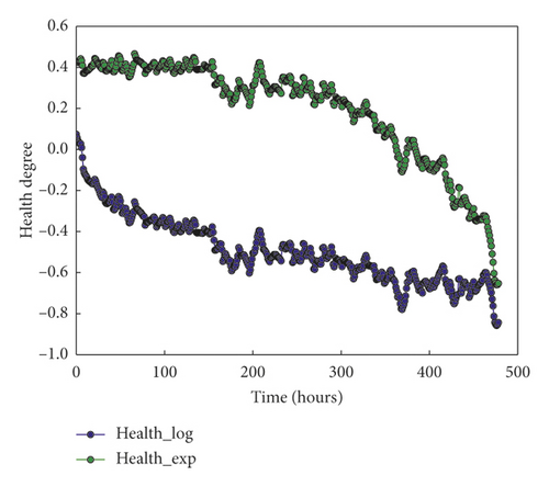
Health degree fluctuates during the degradation of a drive. This phenomenon occurs because the health status change of a drive is influenced by several factors, such as age, IO workload, and environments. To address this issue, we adopt an average smoothing method to reduce the effect of noises on health degree. The average value of health degree, excluding the maximum value and minimum value in the time window [t − (tw/2), t + (tw/2)), is regarded as the health degree at time t, where tw is the size of the smoothing window. Figure 4 shows the smoothing result of health degrees in Figure 3.
4. Experimental Results
To evaluate the effectiveness of our method, we conduct several experiments on two datasets. In this section, we introduce the datasets, experimental setup, evaluation metrics, data preprocessing, and feature selection. Then, we present the experimental results and analysis.
4.1. Datasets
There are two datasets used in our experiments: one is from the Baidu data center [35] and the other is from the Backblaze storage system [36]. The first dataset has 23,395 enterprise-class hard drives, consisting of 433 failed drives and 22,962 good drives. These drives are the same model. According to the replacement log for drives in the data center, a drive was labeled as “failed” or “good.” SMART data from these drives are collected once per hour. For each failed drive, 20-day SMART samples before it failed are used. For good drives, 7-day SMART samples are used. In total, there are 156,312 samples of failed drives and 3,850,141 samples of good drives. The samples in this dataset only have 12 attributes: RSC, SUT, SER, raw read error rate (RRER), reported uncorrectable errors (RUE), high fly writes (HFW), hardware ECC recovered (HER), current pending sector count (CPSC), POH, TC, and the raw data of RSC and CPSC.
The dataset from the Backblaze includes 35,491 desktop-class hard drives with 706 failed drives and 34785 good drives consisting of 80 models from over the course of more than 2 years, which is the largest public SMART dataset. The samples in this dataset were collected once every day. In our experiments, this dataset is separated by the drive model to reduce the impact of different models, as the failure rate and degradation are different across the model and manufacturer [4]. We chose three drive families with the largest number of drives, namely, “ST4000DM000,” “HDS722020ALA330,” and “HDS5C3030ALA630,” for our experimental data. Each sample in these datasets has 24 SMART attributes, and all attributes have a value and raw data. The details of these four drive families are described in Table 1. To clearly describe the experiments, these three drive families are represented as “B1,” “B2,” and “B3,” and the dataset from Baidu is represented as “Baidu.”
| Dataset | Family | Provider | Model | Number of failed drives | Number of good drives | Total number of drives |
|---|---|---|---|---|---|---|
| Baidu | Baidu | Seagate | — | 426 | 22969 | 23395 |
| Backblaze | B1 | Seagate | ST4000DM000 | 706 | 34785 | 35491 |
| B2 | Hitachi | HDS722020ALA330 | 251 | 4468 | 4719 | |
| B3 | Hitachi | HDS5C3030ALA630 | 131 | 4540 | 4671 | |
4.2. Experimental Setup
To simulate the real-life environment of a data center, we built experimental datasets according to the following method: all samples of failed drives were randomly divided into two parts at a ratio of 7 : 3 to ensure the independence of failed drives between the training set and the testing set. Given the deterioration process of drives, we only added the last several samples from the 70% of failed drives before the failure time in the training set. All health samples from the 30% of failed drives were added to the testing set. All samples from good drives were divided into two parts at a ratio of 7 : 3 according to their collection timelines. The earlier health samples were used in the training set, and the later samples were used in the testing set.
Our experiments were trained and tested on a GPU because of the heavy computation overheads of the BPTT algorithm. The GPU model was an NVIDIA Tesla K80, and the server memory was 128G.
4.3. Evaluation Metrics
The ability of HDD failure prediction is usually evaluated and compared based on the FDR, FAR, and lead time. When predicting HDD failure, failed HDDs are regarded as positive drives and good HDDs are regarded as negative drives. True positive drives are failed drives detected by the prediction model before they fail. False positive drives are good drives misclassified as soon-to-fail drives.
We employed high FDRs and low FDRs for our prediction model, but it is difficult for deep learning to achieve both goals at the same time. Hence, we adopt the receive operating characteristic (ROC) curve, which plots the FDR versus FAR. The ROC curve is used to assess the performance of the prediction model to distinguish soon-to-fail drives from good drives. The closer the curve is to the left top corner, the more accurately the model detects soon-to-fail drives.
The lead time is the time span from the moment a HDD was detected as soon-to-fail to the time it actually failed. Users initiate the backup of data in a timely manner if they are alerted. It is necessary for users to be provided sufficient lead time to perform precautionary maintenance, including backing up data and replacing soon-to-fail drives; however, an excessive lead time is meaningless and unnecessarily inflates the reliability overhead. As a result, we adopt the lead time to evaluate the prediction models in the experiments.
4.4. Feature Selection
Some SMART attributes are not strongly correlated with drive deterioration, and retaining these attributes has a negative impact on prediction performance. Hence, we performed feature selection for our experimental datasets. Our feature selection consisted of two steps; the features correlating weakly with drive failure at first were removed, and then some features that describe the change of attributes were added.
Samples in “Baidu” only have 12 features and have been normalized in the public dataset; thus, we did nothing in the first step. For the other dataset, there are approximately 30 attributes for each SMART sample. We introduced the information gain ratio (IGR) to evaluate the importance of each attribute to detect soon-to-fail drives. We chose the attributes with the top 12 IGRs (see Table 2): RSC, RRER (raw read error rate), RRSC, TC, SUT, CPSC, HFW, HER, RCPSC, POH, SER, and RUE for family “B1” and RRSC, RRER, RSC, RCPSC (raw current pending sector count), SRC (spin retry count), SUT, RUE, CT (command timeout), TC, HFW, USC (uncorrectable sector count), POH, and WER (write error rate) for families “B2” and “B3.” From this table, we find that the SMART attributes of drives from different manufacturers are slightly different.
| B1 | B2 | B3 | |||
|---|---|---|---|---|---|
| Attribute | IGR | Attribute | IGR | Attribute | IGR |
| RSC | 0.0326 | RRSC | 0.0413 | RRSC | 0.0339 |
| RRER | 0.028 | RRER | 0.031 | RRER | 0.0327 |
| RRSC | 0.0278 | RSC | 0.0297 | RSC | 0.0262 |
| TC | 0.0277 | RCPSC | 0.0277 | SRC | 0.0231 |
| SUT | 0.0276 | SRC | 0.0271 | SUT | 0.0228 |
| CPSC | 0.0272 | SUT | 0.0251 | RCPSC | 0.0227 |
| HFW | 0.0269 | RUE | 0.0248 | RUE | 0.0214 |
| HER | 0.0251 | CT | 0.0201 | TC | 0.0208 |
| RCPSC | 0.0239 | TC | 0.0189 | WER | 0.0189 |
| POH | 0.0166 | HFW | 0.0161 | CT | 0.0131 |
| SER | 0.0118 | USC | 0.0133 | USC | 0.0129 |
| RUE | 0.0067 | POH | 0.0098 | HFW | 0.0117 |
Some changes of SMART attributes are strongly correlated with the health status of drives [14]. We added some change rates of basic features to improve the performance of the prediction method. For family “Baidu,” we added the 6-hour and 12-hour change rate for all features. For families “B1,” “B2,” and “B3,” we added the 1-day and 2-day change rates of the following attributes: RSC, RRSC, RRER, TC, RCPSC, SER, RUE, SER, WER, and POH.
4.5. Parameter Analysis
Our prediction model has several parameters to optimize: the number of layers in the LSTM-RNN-based model, the size of the sliding window, and the threshold. The results of experiments in this subsection are based on the “Baidu” family as the results in the other families are similar and are limited in length.
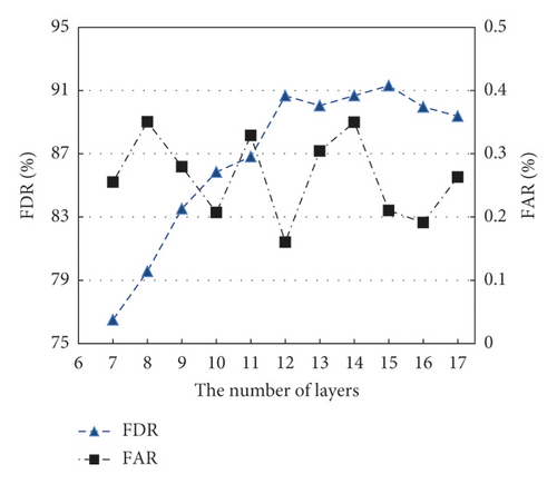
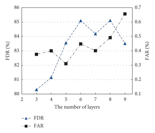
Figure 5 shows the effect of different numbers of layers in the range of 7 to 17 in the LSTM-RNN-based prediction model. When the number of layers is less than 12, the FDR increases steadily but the FAR fluctuates. When the number of layers is more than 12, the FDR no longer increases. The FAR reaches its lowest value at 12 layers. Compared with the LSTM-RNN-based model, the FDR-based model no longer increases when the number of RNN layers is more than 6, as shown in Figure 6.
We tested the influence of different sizes of sliding window and threshold on the prediction performance. The bigger the window size, the higher the FDR and the lower the FAR. Our model achieves the best accuracy when the size of window is set to 14. As the threshold increases, the FDR and FAR both rise. We set the size of window to 14 and the threshold to −0.4 in the following experiments.
There was a serious imbalance issue when training families “Baidu” and “B1” because there are far fewer failed drives than good ones, and not all samples of failed drives were added to the training set. To address this issue, we adopted a k-means-clustering-based undersampling method [14] to reduce the scale of negative samples in the training set. The samples from good drives were clustered into several groups and then sampled from each group. We added good samples at a rate 150 times higher than samples with health degree less than –0.5 of failed drives which were added to the training set for family “Baidu.”
4.6. Comparison and Analysis
In this section, we quantitatively compare the performance of our method with that of widely used models on the Baidu and Backblaze test sets. We focus on the classification and regression tree (CART) and the RNN-based prediction model.
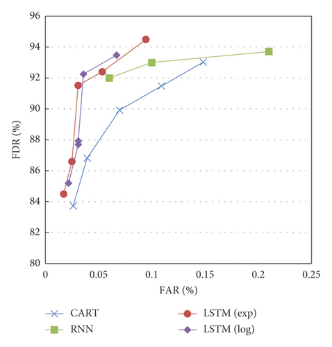
Figure 7 shows the ROC curves obtained by different models for family “Baidu.” Our method outperformed the RNN-based model and the CART-based model. The proposed prediction model achieved an FDR of 94.49% and an FAR of 0.09%. The LSTM-RNN-based model takes advantage of the long dependence feature of drive health data, and health degree evaluation details the drive deterioration and effectively reduces the FARs. The model with exponential function is in general better than the model with logarithmic function. Comparisons of FDRs and FARs for families between different prediction models are shown in Table 3. For “B1,” “B2,” and “B3,” our methods achieved better FDRs than the other models. The CART-based model achieved the lower FARs than the other models. The FARs for family “B2” were worse than those for the other families. And the FARs for family “Baidu” were better than the FARs on families “B1,” “B2,” and “B3” because the interval between samples in the dataset from Backblaze is 24 hours, which is too long to observe the change in health status in the degradation before drive failed.
| Prediction model | B1 | B2 | B3 | |||
|---|---|---|---|---|---|---|
| FDR (%) | FAR (%) | FDR (%) | FAR (%) | FDR (%) | FAR (%) | |
| CART | 76.82 | 0.47 | 68.67 | 1.47 | 63.85 | 0.84 |
| RNN | 73.46 | 0.65 | 68.00 | 2.19 | 66.67 | 1.07 |
| LSTM (Exp) | 79.15 | 0.59 | 77.33 | 2.43 | 79.49 | 0.92 |
| LSTM (Log) | 80.00 | 0.76 | 69.33 | 2.63 | 74.36 | 1.37 |
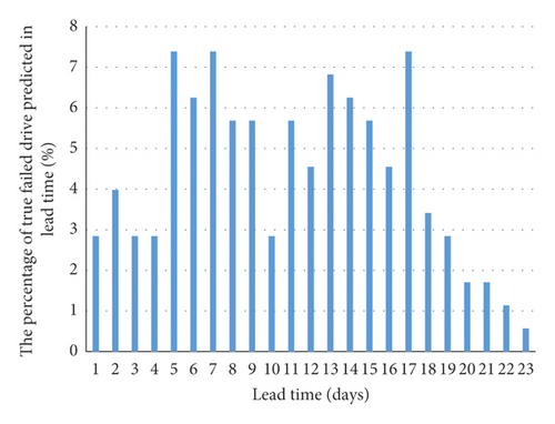
In addition, we compared lead time of these models. Table 4 shows the lead time comparison of prediction models for family “Baidu.” As it can be clearly observed that 100% true positive drives were predicted at 24 hours in advance before they failed. Figures 8 and 9 show that most of drives are predicted by LSTM-RNN-based models at about 7 days in advance before failed. This time allows the backup and data migration process.
| Model | Lead time | ||
|---|---|---|---|
| >24 h (%) | >48 h (%) | >96 h (%) | |
| CART | 90.48 | 67.62 | 0.95 |
| RNN | 100.00 | 83.49 | 33.03 |
| LSTM (Exp) | 100.00 | 93.91 | 41.74 |
| LSTM (Log) | 100.00 | 91.45 | 41.88 |
5. Conclusion
As more and more services are pushed from the cloud to the edge of the network, the high storage reliability on the edge nodes is urgently required, especially in smart surveillance systems. This paper attempts to evaluate the health degree of HDDs to improve the performance of soon-to-fail drive prediction in mobile edge computing environment. An LSTM RNN is employed to extract temporal dependence feature of drive health data and compute the health degree. The deterioration process of drives is greatly influenced by health status, IO workload, and the environment situation. Therefore, a k-means-based undersampling method is used to resolve the problem of data imbalance. It reduces the computation overhead and improves the FDR of the prediction model. We validated our method with two real-life datasets. Comparing with the traditional approaches, the experimental results show that the proposed model achieves the better forecasting performance with a low overhead.
In the future, more analysis of HDD failure can be performed to further enhance the prediction accuracy and make prediction models intelligent enough to provide effective instructions and suggestions.
Conflicts of Interest
The authors declare that they have no conflicts of interest.
Acknowledgments
The work described in this paper was supported by the Fund of the Natural Science Foundation of Zhejiang Province (no. LQ17F020004) and Open Research Fund of State Key Laboratory of Computer Architecture. The authors also thank Baidu Inc. and BackBlaze Inc. for providing the datasets used in this work.
Open Research
Data Availability
The data used in the experiments of this study are available in Baidu and Backblaze. These data were derived from the following resources available in the public domains: http://pan.baidu.com/share/link?shareid=189977&uk=4278294944 and https://www.backblaze.com/b2/hard-drive-test-data.html#downloading-the-raw-hard-drive-test-data.


