Image matching is a method of matching by analyzing the gray scale and texture information of the reference image and the image to be matched. Firstly, the scale invariant feature transform (SIFT) algorithm has long descriptor time and poor real time, a nonlinear dimension reduction method (LLE) based on local linear embedding is proposed to preserve the nonlinear information in the original data space as much as possible, shorten the running time of the algorithm, and improve the matching accuracy. Second, aiming at the problem that the Euclidean distance takes a large amount of calculation in the matching process, Manhattan distance is proposed to calculate the similarity between the reference image and the image to be matched, so as to further reduce the algorithm time. Through the improved LLE-SIFT algorithm, experimental results show that the algorithm has a high matching rate and improves the matching speed.

1. Introduction

The development of image recognition has experienced three stages: text recognition, digital image processing and recognition, and object recognition. With the continuous development of modern science and technology, various application fields of image matching have increasingly high requirements on its performance, such as reducing the difficulty of the matching algorithm, improving the accuracy of the algorithm, and reducing the matching time. At the same time, the image is easy to be affected by lighting, equipment, natural environment changes, and other conditions during the shooting process, and the image is no longer only a simple two-dimensional form [1], but a three-dimensional or even multidimensional form. Ensuring the matching accuracy of the image under these circumstances has become the focus of research. Object recognition mainly refers to the perception and understanding of the object and environment of the three-dimensional world, which belongs to the category of advanced computer vision. It is based on digital image processing and recognition combined with artificial intelligence, system science, and other disciplines research direction; its research results have been widely used in a variety of industrial and detection robots. One of the shortcomings of modern image recognition technology is its poor adaptive performance. Once the target image is polluted by strong noise or has a large defect, it often cannot get the ideal result.

1.1. Research Status

The main method of matching based on the transform domain is the Fourier transform method, which has the following advantages: the translation, rotation, affine, and other transformations of the image are reflected in the Fourier transform domain. It is also possible to obtain a certain degree of robustness against noise using the transform domain method. Owing to the mature fast algorithm and easy hardware implementation, Fourier transform has its unique advantages in algorithm implementation.

The matching algorithm based on feature detection is more powerful and comprehensive. In addition to having a better matching effect on the image with translation transformation and rotation transformation, it also has a better performance on the matching between the image with affine transformation and projection transformation. It consists of three steps: feature point detection, feature description operator calculation, and feature point matching. The main feature point detection algorithms include Harris corner detection, SIFT feature detection, and SUSAN feature point detection. These algorithms can detect the location of feature points in the image. Moreover, as feature-based image matching algorithm only describes and matches some information-rich regions in the image, its computational amount is far less than that of image matching algorithm based on gray scale, so it is widely used in the fields requiring high real-time performance.

Moravec proposed the Moravec algorithm, which used the autocorrelation function to extract key information from the image. Harris and Stephen improved Moravec corner detection algorithm and proposed a Harris corner detection algorithm, which has certain rotation invariance and has certain robustness to the influence of light and noise [2]. Lowe et al. proposed SIFT descriptors and perfected SIFT feature matching algorithm, which is robust to rotation changes, scale changes, and illumination changes, and is widely used in many fields due to its excellent performance [3]. The PCA-SIFT proposed by Ke and Sukthankar reduces the matching time by reducing the dimensions of SIFT descriptors [4]. Liu proposed the FAST-SIFT, using FAST algorithm to calculate the feature points of the image to be tested and SIFT descriptor description to improve the efficiency of SIFT feature matching algorithm [5]. In view of the long calculation time caused by the high dimension of SIFT feature descriptors, Yang Jianwen [6] used DAISY, FREAK, and other binary descriptors to replace SIFT descriptors and used coarse matching and fine matching to improve the matching accuracy. In view of the poor matching performance of SIFT algorithm for image flipping photos, Ma Yan, Su Mingzhe, and Zhang Xiangfen et al. [7] put forward an MBR-SIFT descriptor. The SIFT algorithm, by carrying out binarization and other operations on reconstructed SIFT descriptor, while retaining the senior robust characteristics, also has the robustness of mirror flipping [8]. Barnea and Silverman changed the detection window of value points to 5 ∗ 5 and replaced the processing window for generating feature descriptors with a 12-ring circular region, which reduced the calculation time of image matching steps [9].

The accuracy of feature extraction directly affects the accuracy of image matching, so feature extraction is the key step of feature-based image matching algorithm. Based on gray scale, the image matching algorithm uses the idea of statistics to abstract the image into a two-dimensional signal, convert the matching between the images into correlation matching between the signals, and determine the similarity of the two signals through the correlation function, so as to determine the point with the same name [10]. The currently used methods are the average absolute difference (MAD) algorithm, sequence similarity detection (SSDA) algorithm, normalized cross correlation (NCC) algorithm, and so on.

The mean absolute difference (MAD) algorithm is proposed by Leese. The MAD algorithm matches the subgraph of the image to be tested by comparing the mean absolute difference with the template [11]. Ouyang et al. proposed the sequence similarity detection algorithm (SSDA). Compared with the MAD algorithm, the SSDA algorithm can complete the matching without traversal of the whole image, which reduces the amount of computation and is a relatively easy algorithm to implement [12]. Rosenfeld and Kak proposed the normalized cross-correlation (NCC) algorithm, which used a normalized similarity measurement formula to detect the gray levels of the subgraph and the template image respectively, so as to obtain the matching degree between the two images. NCC algorithm is considered to have the best performance among the image matching algorithms based on gray level [13]. Zagoruyko and Komodakis [14] used integral and square integral images to simplify the addition and subtraction of pixel values in the processing window to the addition and subtraction of four pixel points, which reduces the search scope and improves the real-time performance of NCC algorithm. Melekhov et al. [15] used the method of retaining image feature information to reduce the redundant information of the template to improve the generation and search speed of the template and improve the efficiency of the NCC algorithm.

In general, the image matching method based on gray level has a good matching accuracy rate, but due to its large amount of calculation, the matching efficiency is low, and it cannot be applied in some fields requiring high real-time performance.

1.2. Contents and Methods

Image recognition technology can be divided into two types of image recognition systems according to image types: one is the human image recognition system, with a high level of artificial intelligence technology. The other is the computer image recognition system, with high computational efficiency. The difference between these two forms in practical application is small, and the classification is not particularly obvious [16]. The main difference between them is that the computer image recognition technology is not affected by human sensory differences and other factors. However, in the human image recognition system due to the humanized processing learning concept and growth algorithm, the complex image can be processed at different levels of information.

Image data set dimension reduction is an operation to transform a single image into a data set in a high-dimensional space through high-dimensional transformation of a single image data. In machine learning, dimension reduction refers to the use of some mapping method to map the data points in the original high-dimensional space to the low-dimensional space. The essence of dimension reduction is to learn a mapping function f: x⟶y, where x is the expression of original data points, and the vector expression form is most used at present. y is a low-dimensional vector representation of the data points mapped [17]. In general, the dimension of y is less than the dimension of x (of course, it is possible to increase the dimension). f may be explicit or implicit, linear or nonlinear. As the dimensions of the data decrease, less space is needed to store the data, and low-dimensional data can help reduce computing or training time. Some algorithms tend to perform poorly on high-dimensional data. Dimension reduction can improve the availability of algorithms. In addition, dimension reduction can solve the multicollinearity problem by removing redundant features, which is helpful for data visualization. If the dimensions of the data are very high, visualization becomes quite difficult, whereas drawing two- and three-dimensional data is simpler [18].

This paper mainly studies manifold learning-based image dimension reduction algorithm and feature-based image matching algorithm. Its core idea is to represent multidimensional images in dimension reduction, and the process of dimension reduction is shown in Figure 1:

Details are in the caption following the image — **Figure 1**
Open in figure viewer PowerPoint

Image dimension reduction process.

Next, the feature space of different images is calculated, and the similarity of features in the feature space is measured, so as to complete the matching between the images. The matching process is shown in Figure 2:

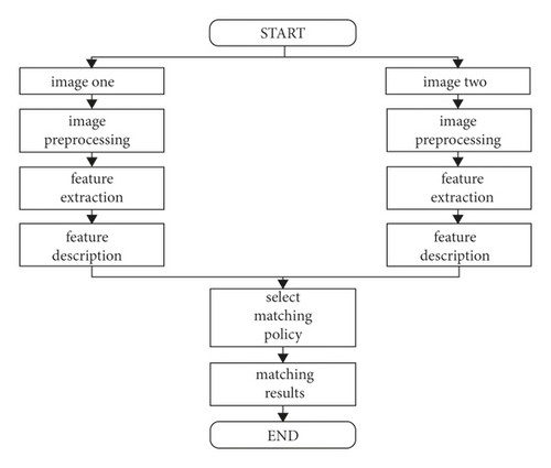
It is not difficult to see from Figure 2 that feature-based image matching only describes and matches some information-rich regions in the image, so its computation is small.

2. Algorithm Model

With the development of data acquisition tools, such as sensors and high-definition cameras, as well as the needs of real life, the traditional image acquisition field often has to deal with a large amount of high-dimensional data. Although the high-dimensional data preserve the structure information of the image to a certain extent and ensure the accuracy of the extraction of image features and data restoration, the high-dimensional data are not easy to be perceived and understood. Moreover, the disaster of dimension brought by the high-dimensional data greatly increases the complexity of calculation. In view of this situation, manifold learning has become a major research direction of image dimension reduction in recent years [19]. The essence of manifold learning is to find the corresponding low-dimensional manifold structure with some embedded mapping for those low-dimensional manifold data with higher-dimensional Euclidean space properties. The reason why data can be mapped from high dimensions to low dimensions is that the high-dimensional data used in our daily life are limited by internal attributes, resulting in the redundancy of dimensions, and only low dimensions can represent data features [20].

2.1. Principle and Classification of Manifold Learning

The six basic elements of manifold learning are as follows: observation of high-dimensional data, selection of appropriate intrinsic dimension, low-dimensional representation of high-dimensional data, embedding mapping of manifold, reconstruction mapping to data recovery, and restriction condition of filtering noise.

Manifold learning assumes that high-dimensional data have a low-dimensional manifold, which can contain most of the information of the data. Through certain mapping and perception, the original high-dimensional data are mapped to the low-dimensional embedding space, and the low-dimensional embedding space retains the internal associations and geometric attributes of the original data.

Suppose the high-dimensional observation data are: x = {x_i ∈ R^D, i = 1, L, N}, where N is the data volume of a given sample, and D is the dimension of high-dimensional data. Suppose there is a low-dimensional manifold expressed as Ω^D⊆R^D, the intrinsic dimension is d(d < D&d ≪ D). The purpose of image dimension reduction in manifold learning is to find out the mapping relationship from high-dimensional data to low-dimensional embedding space, which is expressed as f, so that y_i = f(x_i), so as to obtain the low-dimensional representation y_i ∈ R^D of high-dimensional data x_i. In the data reconstruction and recovery stage, in order to restore the original image with maximum accuracy and retain the geometric structure of the original manifold data, the original data x_i = f⁻¹(y_i) can be restored according to the y_i = f(x_i) mapping function f, which needs to meet specific restrictions.

Manifold learning can have different classification methods according to different constraints and feature extraction criteria. The most common is to classify manifolds according to their structural characteristics. There are two ways:

(1)
Linear analysis: Linearity means that the mapping function f satisfies the linear relationship, including principal component analysis, multiscale transformation, and linear discrimination. For example, two-dimensional principal component analysis (2DPCA), its theme is to find the underdetermined linear mapping matrix y, y = ϕ₁xϕ₂, on the row or column of the original data x. Since the line maps ϕ₁ and ϕ₂ are nonrandom underdetermined matrices, the columns and columns of the compressed matrix y are less than the columns and columns of x.
(2)
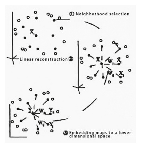
Nonlinear analysis: As a special form of nonlinear analysis method, the main disadvantage of linear analysis method is that when the data dimension is very high, the calculation of eigenvector becomes infeasible. Due to the uncertainty of data distribution and dispersion, nonlinear analysis assumes that the data are located in a low-dimensional nonlinear manifold, and then starting from the local neighbor structure of data, the manifold learning problem is transformed into the objective function of optimization problem, by solving the objective function to draw manifold geometric properties of data needed to keep, namely underdetermined mapping matrix. Then the low-dimensional embedded representation of the original high-dimensional data is obtained. A typical method is local linear embedding (LLE), as shown in Figure 3.

For each data point, i = 1,2, L, N of sample data x_i, k nearest neighbors x_ij are defined within the scope of its domain, and the reconstruction error is defined as

(1)

where W_ij represents the weight between x_i and x_ij. When

, the local optimal reconstruction matrix can be obtained by Lagrangian operator:

(2)

Qⁱ is the singular matrix, and the mapping conditions for mapping high-dimensional data to low-dimensional space are

(3)

where y_i is the output vector of x_i and ε(Y) is the function value lost during data reconstruction. The nonlinear analysis method preserves the geometric structure relations between domains and can also map the rotation, translation, and expansion of neighbor weights of domain points. Therefore, the nonlinear analysis method can keep the invariance of manifold structure well.

2.2. Intrinsic Dimension Estimation

On the premise of not reducing the accuracy of image restoration, the low-dimensional representation of high-dimensional data is obtained by manifold learning mapping, thus reducing the computational complexity. The intrinsic dimension estimation solves the problem of how to accurately restore the original data with the least data structure. The intrinsic dimension estimation contains all the information of the data set and does not change with the change of the mapping matrix. It can represent all the information of the data set with the least free parameters. Only the proper intrinsic dimension estimation can play a positive role in image reconstruction. If the intrinsic dimension estimation is too small, the result after dimension reduction cannot be guaranteed to contain enough eigenvector length for image reconstruction. If the intrinsic dimension estimation is too large, there will be a lot of redundant noise in the result of dimension reduction, which will affect the accuracy of image reconstruction. Therefore, the estimation of the intrinsic dimension estimation is very important.

There are two kinds of intrinsic dimension estimation: one is to estimate the local geometric features of high-dimensional data using geometric methods. The other is the eigenvalue method for linear data, which is an estimate of the global intrinsic dimension estimation. In view of the characteristics of manifold learning, the advantages of using geometric methods to estimate the intrinsic dimensions have attracted more and more attention. There are two common methods for estimating intrinsic dimension:

2.2.1. K-Nearest Neighbor (KNN)

Let y_n = {Y₁, LY_n} be an independent random sample in space R^D, and take y_n as a vertex. For any point, connect all its k-neighbors and get the k-neighbor graph. Through all k-neighbor combination of Y_i is N_k,i = N_k,i(y_n), the total length of internal edges of k-neighbor graph can be obtained as follows:

(4)

Assume a compact m-dimensional manifold (m, g) and take the limit of the total length of the internal edges:

(5)

where β_m,r,k is a constant independent of f, satisfying α = (m − r)/m if and only if d^′ = m.

Let l_n = log L_r,k(y_n), through the approximation condition

(6)

where a = (m − r)/m,

, and ε_n is the variance.

is a finite value whose limit value is nonzero:

(7)

By sorting out the above formulas and concepts, the intrinsic dimension of the data set is estimated as

(8)

where

is the linear mean square estimate of a and r > 0 is the weight constant.

2.2.2. Maximum Likelihood Estimate (MLE)

Random sampling sample X₁, LX_n is selected from the space R^D, and a point x is taken as the center and a circle is made with R as the radius, then the number of samples of sample X₁, LX_n in the sphere is

(9)

The distance from the kth nearest neighbor of x to x in sample X₁, …, X_n:

(10)

For a nonstationary process with fixed t, the parameters of Poisson process are

(11)

Establish the likelihood function for Poisson process

(12)

Take the partial derivative of the likelihood function, and then obtain the maximum likelihood estimate:

(13)

The intrinsic dimension can be obtained from the above equation:

(14)

2.3. Scale-Invariant Feature Transform (SIFT)

SIFT is an image matching algorithm proposed and improved by Lowe in 2004, including the following steps:

(1)
Establish scale space: Using Gaussian convolution kernel function to construct scale space (scale space is real).
(2)
Detect extreme points: Gaussian pyramid was constructed through the establishment of scale space, and the DOG Gaussian difference pyramid was constructed by subtracting the two adjacent layers of each group of Gaussian pyramid. Extreme points were detected in the constructed DOG pyramid. A total of 26 points were compared between each sampling point and 8 points in the neighborhood of the same layer and 9 points in the upper and lower layers by the traversal method to verify whether it was an extreme point. If it was, it was a potential feature point.
(3)
Locate feature points accurately: After obtaining potential feature points, low-contrast feature points and edge response points are screened out to purify the feature points. Low contrast points are excluded by finding the extreme value of the Taylor expansion of the DOG function and discarding the feature points whose absolute value of the extreme value is less than 0.03. Hessian matrix properties at the feature points are used to exclude the edge response points.
(4)
Distribute direction of feature points: Make a gradient histogram for the neighborhood of feature points, and every 10° is an equal part. The angle corresponding to the highest point of the final histogram is the main direction of the feature points, and the angle reaching 80% of the peak is the auxiliary direction.
(5)
Establish descriptors: Lowe proposed to divide the neighborhood of feature points into 4 × 4 subregions, each subregion containing 8 directions, so each feature point could be represented by 4 × 4 × 8 = 128 dimensional vector.

3. Improved Algorithm

3.1. Manifold Learning Algorithm for Sparse Representation

According to the sparse representation theory, if the information of an image data set is concentrated in a manifold or has sparsity under a certain transformation (that is, the zero element terms of the vector are the majority), then the image data can be obtained through the underdetermined random mapping based on this sparsity, and the compressed data of the image can be obtained without worrying about the loss of any information. Let the image x be a matrix of M × N, and the matrix is transformed into the column vector x^(vec) ∈ R^M×N, then the vector feature y^(vec) ∈ R^M(vec) in the form of one-dimensional compressed sampling of the image can be obtained by the following equation:

(15)

where Φ ∈ R^M(vec)×(MN)(M^(vec) < MN) is an underdetermined random matrix satisfying the RIP condition (Gaussian distribution can be used as the random distribution).

(16)

The data collection method of sparse representation is shown in Figure 4.

3.2. Sparse Local Linear Embedding

As the main manifold learning algorithm, the local linear embedding (LLE) has great advantages in processing high-dimensional data and noniterative method, and LLE can completely reflect the internal distribution of data. However, this is achieved under the premise that the data is in a smooth manifold. Once the manifold is distorted or the number of samples is insufficient, the local embedding method cannot achieve accurate data extraction.

Aiming at these two shortcomings of the local embedding method, the Sparse Local Linear Embedding (SLLE) is proposed. By modifying the modeling objective function of LLE for local regions, SLLE introduces sparse constraints. After sparse constraint optimization of local linear embedding, samples can be reconstructed in low-dimensional space using the weight (sparsity) optimized in high-dimensional space and then the manifold structure of samples can be restored.

The Sparse Local Linear Embedding (SLLE) process:

(1)
Input N m-dimension experimental sample A = [Y₁, Y₂L, Y_N] ∈ R^m×N, error ε > 0.
(2)
The experimental sample A = [Y₁, Y₂L, Y_N] ∈ R^m×N is optimized with 2-norm to generate random matrices Φ ∈ R^m×m, Y = ΦA, and a new sample set .
(3)
Set and convert it into a 1-norm optimization problem: .
(4)
Repeat Step 3 for the sample set. The weight vector of the ith sample is W_i = [W_i1, W_i1K0, KW_in], and the weight of the ith sample is W_ij = 0.
(5)
The weight solution is fixed, and the low-dimensional neighborhood reconstruction error is minimized.
(6)
Final output: X = argminε(X).

In view of the problem that SIFT matching takes a long time, we propose a SIFT algorithm based on local linear embedding (LLE) method (hereinafter called LLE-SIFT). Compared with PCA-SIFT, which can only reduce dimension linearly, the improved algorithm also considers the local nonlinear relationship of the descriptor. On this basis, Manhattan distance is used to replace Euclidean distance as the matching similarity criterion, which reduces the time complexity of the algorithm. The experimental results show that the algorithm can not only guarantee the high matching rate but also improve the image matching speed.

3.3. LLE-SIFT Process

Step 1. Simplify the descriptor:

(1)
The region with the scale of 41 × 41, where the feature points are located, is taken as the domain, and the gradient is calculated (the outermost layer is not calculated), and the 39 × 39 × 2 = 3042 dimensional vector is obtained. Therefore, the descriptor X for each feature point is X = [x₁, …, x_i, …, x₃₀₄₂] (x_i is a dimension in descriptor X), k nearest neighbor points from x_i are found according to the Euclidean distance between two pairs.
(2)
The reconstruction weight W is calculated according to the nearest neighbor points of each descriptor, where the ith dimension can be expressed as
(17)
Solving the weight coefficient matrix W can be transformed into an optimization problem by solving the following:
(18)
(3)
The weight coefficient of the low-dimensional space is shared with that of the high-dimensional space. The output vector Y of the corresponding low-dimensional space is calculated by the weight coefficient matrix W and its nearest neighbor x_ik. Let Y = [y₁, …, y_n] construct the following optimization problem:
(19)
Therefore, we only need to determine the number of the nearest neighbor points and the final dimension to obtain the feature descriptor after dimension reduction. Different from the dimension vector obtained by PCA-SIFT algorithm, the data obtained by LLE-SIFT retained the local nonlinear information in the high-dimensional vector, so when the image is nonlinear processing, better matching effect can be obtained using this algorithm.

Step 2. Improve similarity criterion:

In this paper, Manhattan distance is used to replace Euclidean distance as a criterion to measure the similarity of image features, and Manhattan distance between n-dimensional vectors is defined as

(20)

where r_j and s_j are respectively the descriptors of a feature point of the reference image and the image to be matched. According to the definition, the calculation of Manhattan distance is much less than that of the Euclidean distance. SLLE, the model proposed in this paper, is used to reduce the dimension of the descriptor. Experimental verification shows that the comprehensive effect is best when the descriptor is reduced to 36 dimensions. After dimension reduction, the descriptor of the feature point in the reference graph is expressed as R_i = (r_i1, …, r_i36), and the descriptor of the feature point in the graph to be matched is S_i = (s_i1, …, s_i36). Manhattan distance ratio relationship of the feature descriptor is used to judge the similarity of the feature points in the two images. If it satisfies equation (21), it is considered to be the correct matching point; otherwise, it is the wrong matching point. The best effect is achieved when the threshold value of Lowe is set between 0.4 and 0.8. In the experiment in this paper, the threshold value is set at 0.6. As follows:

(21)

4. Experiment and Discussion

In order to ensure the universal applicability of the algorithm, a lot of experimental verification was carried out in this paper, including the addition of Gaussian white noise with different variances, rotation and scale changes to the image, and the traditional SIFT algorithm, PCA-SIFT algorithm, and the improved algorithm in this paper were respectively used for image matching. The matching logarithm, matching accuracy, and matching time were compared and analyzed.

4.1. Experiment A

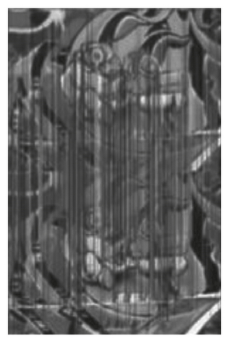
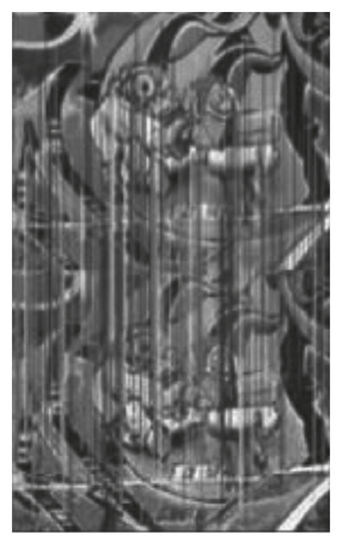
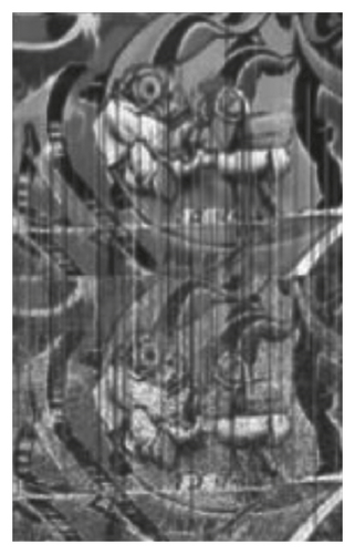
This part of the experiment is mainly to compare the performance of different algorithms under different White Gaussian noise. White Gaussian noise with different variances (S represents standard deviation) was added to the original image, and S values were 10, 20, 40, and 80 in the experiment. The matching results of White Gaussian noise with different variances under LLE-SIFT are shown in Figure 5. The comparison of the algorithms is shown in Table 1. It can be seen from the table that the more White Gaussian noise, the lower the correct matching rate of the three algorithms, but LLE-SIFT has the highest matching accuracy and the shortest matching time when faced with different White Gaussian noise. (For the convenience of display, the comparison result factors in the table are represented by letters: NMK represents the matching logarithm, NCMK represents the correct matching logarithm, RCM represents the correct matching rate, and T represents the matching time (unit: s)).

Table 1. Performance of each algorithm under different noises.

Algorithm	σ = 10				σ = 20				σ = 40				σ = 80
Algorithm	NMK	NCMK	RCM (%)	T (s)	NMK	NCMK	RCM (%)	T (s)	NMK	NCMK	RCM (%)	T (s)	NMK	NCMK	RCM (%)	T (s)
SIFT	782	587	75.1	11.22	638	432	67.7	9.58	536	321	59.9	8.55	186	98	52.7	5.26
PCA-SIFT	626	483	77.2	7.63	506	348	68.8	6.45	388	242	62.3	5.27	151	88	58.3	4.14
LLE-SIFT	591	474	80.2	5.72	440	335	76.1	4.29	292	203	69.5	3.78	114	70	61.4	2.82

4.2. Experiment B

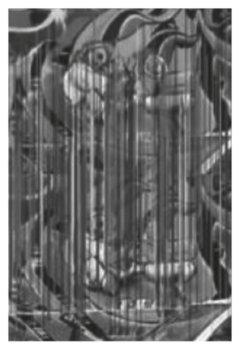
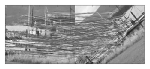
This part of the experiment is mainly to compare the performance of each algorithm under rotation and scale change. The right side of Figure 6 is the image obtained after 30° rotation and scaling of the original image (the left side of Figure 6). Figure 6 is the effect diagram of feature matching using LLE-SIFT algorithm. The comparison of various algorithms is shown in Table 2, indicating that LLE-SIFT algorithm performs better.

Table 2. Rotation and scale change of each algorithm.

Algorithm	NMK	NCMK	RCM/%	T/s
SIFT	363	297	81.8	7.76
PCA-SIFT	328	263	80.2	5.34
LLE-SIFT	396	269	90.0	3.18

4.3. Experiment C

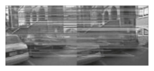
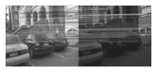
This part of the experiment is mainly to compare the performance of each algorithm under light change. In the matching scene, it is difficult to ensure that the illumination brightness of each image is consistent, so the matching effect of each algorithm under different illumination is especially important. Figure 7 shows the result of LLE-SIFT for image feature matching under different illumination. The comparison of these algorithms is shown in Table 3, and it can be seen that LLE-SIFT has the best performance.

Table 3. Performance of each algorithm under illumination variation.

Algorithm	High light				Low light
Algorithm	NMK	NCMK	RCM (%)	T (s)	NMK	NCMK	RCM (%)	T (s)
SIFT	392	316	80.6	5.22	146	90	61.6	4.46
PCA-SIFT	347	284	81.8	4.31	99	67	67.7	4.03
LLE-SIFT	313	279	89.1	2.06	84	59	70.2	1.57

As can be seen from Tables 1 and 3, both PCA-SIFT and LLE-SIFT proposed in this paper have well inherited the robustness of SIFT for noise, illumination, and other disturbances. However, PCA method is a linear dimension reduction method, which indicates that part of nonlinear information will be lost in the process of dimension reduction, resulting in the decrease of matching accuracy. As shown in Table 2, when the image is rotated, the accuracy of PCA-SIFT decreases by 1.6% compared with SIFT algorithm, while LLE-SIFT improves by 8.2%.

5. Conclusion

First, in view of the problems existing in the process of matching SIFT algorithm, such as time-consuming, the real-time character, in this paper, on the basis of the SIFT algorithm, considering the relationship between the local nonlinear descriptor, LLE in using manifold learning algorithm is proposed for feature point descriptor dimension reduction, and the use of alternative Euclidean distance as Manhattan distance matching similarity criterion, the time complexity of the algorithm is reduced, and the LLE-SIFT algorithm is improved.

Next, we did three sets of experiments. Under the processing of different White Gaussian noise, rotation, and varying scale, LLE-SIFT algorithm has better matching accuracy and performance than other algorithms. It has the highest matching accuracy and the shortest matching time. Experiments show that LLE-SIFT algorithm can improve the image matching speed and save the image matching time while ensuring a high matching rate.

Finally, the results show that LLE-SIFT algorithm not only retains high matching accuracy and good robustness but also saves the matching time and meets the real-time requirements. Compared with SIFT algorithm, it is a better image matching algorithm.

Although deep learning has had great success in image recognition so far, there are still many challenges to be faced before it can be further widely used. Challenge 1: How to improve the generalization capability of the model. Challenge 2: How to leverage small and very large-scale data. Challenge 3: Relationship modeling also has great research potential.

Conflicts of Interest

The author(s) declare no potential conflicts of interest with respect to the research, authorship, and/or publication of this article.

Acknowledgments

This work was supported by the State Grid Corporation Headquarters Technology Project (project title: Research and Application of Substation High-definition Video and Robot Joint Inspection Technology Based on Multidimensional Image Intelligent Matching and Recognition Technology; grant no. 5500-202017083A-0-0-00).

Open Research

Data Availability

The data that support the findings of this study are available from the corresponding author upon reasonable request.

References

1 Moracec H. P., Towards Automatic Visual Obstacle Avoidance, International Joint Conference on Artificial Intelligence, 1977, Morgan Kaufman Publisher Inc., Burlington, MA, USA.
Google Scholar
2 Cui Z., Image Feature Point Extraction and Matching Based on SIFT Algorithm, 2016, University of Electronic Science and Technology of China, Chengdu, China.
Google Scholar
3 Lowe D. G., Distinctive image features from scale-invariant keypoints, International Journal of Computer Vision. (2004) 60, no. 2, 91–110, https://doi.org/10.1023/b:visi.0000029664.99615.94, 2-s2.0-3042535216.
10.1023/B:VISI.0000029664.99615.94
Web of Science® Google Scholar
4 Ke N. Y. and Sukthankar R., PCA-SIFT:a more distinctive representation for local image descriptors, Proceedings of the IEEE Computer Society Conference on Computer Vision & Pattern Recognition, June-July 2004, San Francisco, CA, USA, IEEE Computer Society.
Google Scholar
5 Liu P. F., Research on Image Registration Method Based on SIFT, 2019, Harbin Institute of Technology, Harbin, China.
Google Scholar
6 Yang J. W., Research on Improved Oblique Image Matching Based on SIFT, 2019, China University of Mining and Technology, Xuzhou, China.
Google Scholar
7 Lu Q., Research and Evaluation of Improved Image Mosaic Algorithm Based on SIFT, 2019, Shanghai Ocean University, Shanghai, China.
Google Scholar
8 Ma Y., Su M. Z., and Zhang X. F., Image Matching Method Based on MBR-SIFT Descriptor, 2018, Shanghai Normal University, Shanghai, China.
Google Scholar
9 Barnea D. I. and Silverman H. F., A class of algorithms for fast digital image registration, IEEE Transactions on Computers. (2009) C-21, no. 2, 179–186.
10.1109/TC.1972.5008923
Google Scholar
10 Rosenfeld A. and Kak A. C., Digital picture processing-volume 1, volume 2, Computer ENCE & Applied Mathematics. (1982) 6, no. 2, 113–116.
Google Scholar
11 Wang E. G. and Wu S. F., Fast matching algorithm of NCC edge information, Electronic Technology. (2007) 12, 19–21.
Google Scholar
12 Ouyang X. Y., Zhang J. J., and Zhao N. N., Improved stereo matching algorithm based on MCC, Microcomputer & Its Applications. (2015) no. 3, 54–57.
Google Scholar
13 Wang X. Y., Huang Y. F., Zhu H. J., and Jiang H. F., Study on variable lane control method application in ITS, Basic and Clinical Pharmacology and Toxicology. (2019) no. 10, 14–22.
PubMed Web of Science® Google Scholar
14 Zagoruyko S. and Komodakis N., Learning to compare image patches via convolutional neural networks, Proceedings of the IEEE Conference on Computer Vision and Pattern Recognition (CVPR), June 2015, Boston, MA, USA, 4353–4361, https://doi.org/10.1109/cvpr.2015.7299064, 2-s2.0-84959179619.
10.1109/cvpr.2015.7299064
Google Scholar
15 Melekhov I., Kannala J., and Rahtu E., Siamese network features for image matching, Proceedings of the 23rd International Conference on Pattern Recognition (ICPR), December 2016, Cancun, Mexico, 13–18.
Google Scholar
16 Simonyan K. and Zisserman A., 2014, Verydeepconvolutionalnetworksforlarge-scaleimagerecognition.
Google Scholar
17 Sun Y., Zhu L., Wang G., and Zhao F., Multi-input convolutional neural network for flower grading, Journal of Electrical and Computer Engineering. (2017) 8, https://doi.org/10.1155/2017/9240407, 2-s2.0-85029813473.
10.1155/2017/9240407
Google Scholar
18 Varga D. and Szirányi T., Fast content-based image retrieval using convolutional neural network and hash function, Proceedings of the 2016 IEEE International Conference on Systems, Man, and Cybernetics (SMC), October, 2016, Budapest, Hungary, 2636–2640, https://doi.org/10.1109/smc.2016.7844637, 2-s2.0-85015726916.
10.1109/smc.2016.7844637
Google Scholar
19 Liu H., Tian Y., Wang Y., Pang L., and Huang T., Deep relative distance learning: tell the difference between similar vehicles, Proceedings of the IEEE Conference on Computer Vision and Pattern Recognition (CVPR), July 2016, Las Vegas, NV, USA, 2167–2175, https://doi.org/10.1109/cvpr.2016.238, 2-s2.0-84986278256.
10.1109/cvpr.2016.238
Google Scholar
20 Jiang H., Han A Q., Wang M. J., Wang Z., and Wu Y. L., Solution algorithm of stringsimilarity based on improved Levenshtein distance, Comput. Eng.(2014) 40, no. 1.
Google Scholar

Citing Literature

All articles

Research on Multidimensional Image Intelligent Matching Algorithm of Artificial Intelligence Image Recognition Technology

Abstract