Volume 2021, Issue 1 6251399

Research Article

Open Access

Multitarget Vehicle Tracking and Motion State Estimation Using a Novel Driving Environment Perception System of Intelligent Vehicles

Yuren Chen

The Key Laboratory of Road and Traffic Engineering, Ministry of Education, Tongji University, Shanghai 201804, China moe.edu.cn

Shanghai Institute of Intelligent Science and Technology, Tongji University, Shanghai 201804, China tongji.edu.cn

Search for more papers by this author

Xinyi Xie,

Xinyi Xie

The Key Laboratory of Road and Traffic Engineering, Ministry of Education, Tongji University, Shanghai 201804, China moe.edu.cn

Search for more papers by this author

Bo Yu,

Corresponding Author

Bo Yu

[email protected]

orcid.org/0000-0003-3101-3907

The Key Laboratory of Road and Traffic Engineering, Ministry of Education, Tongji University, Shanghai 201804, China moe.edu.cn

Search for more papers by this author

Yi Li,

Yi Li

Logistics Research Center, Shanghai Maritime University, Haigang Ave. 1550, Shanghai, China shmtu.edu.cn

Search for more papers by this author

Kunhui Lin,

Kunhui Lin

The Key Laboratory of Road and Traffic Engineering, Ministry of Education, Tongji University, Shanghai 201804, China moe.edu.cn

Search for more papers by this author

Yuren Chen,

Yuren Chen

The Key Laboratory of Road and Traffic Engineering, Ministry of Education, Tongji University, Shanghai 201804, China moe.edu.cn

Shanghai Institute of Intelligent Science and Technology, Tongji University, Shanghai 201804, China tongji.edu.cn

Search for more papers by this author

Xinyi Xie,

Xinyi Xie

The Key Laboratory of Road and Traffic Engineering, Ministry of Education, Tongji University, Shanghai 201804, China moe.edu.cn

Search for more papers by this author

Bo Yu,

Corresponding Author

Bo Yu

[email protected]

orcid.org/0000-0003-3101-3907

The Key Laboratory of Road and Traffic Engineering, Ministry of Education, Tongji University, Shanghai 201804, China moe.edu.cn

Search for more papers by this author

Yi Li,

Yi Li

Logistics Research Center, Shanghai Maritime University, Haigang Ave. 1550, Shanghai, China shmtu.edu.cn

Search for more papers by this author

Kunhui Lin,

Kunhui Lin

The Key Laboratory of Road and Traffic Engineering, Ministry of Education, Tongji University, Shanghai 201804, China moe.edu.cn

Search for more papers by this author

First published: 15 September 2021

https://doi.org/10.1155/2021/6251399

Citations: 4

Academic Editor: Yanyong Guo

Share a link

Email
Wechat
Bluesky

Abstract

The multitarget vehicle tracking and motion state estimation are crucial for controlling the host vehicle accurately and preventing collisions. However, current multitarget tracking methods are inconvenient to deal with multivehicle issues due to the dynamically complex driving environment. Driving environment perception systems, as an indispensable component of intelligent vehicles, have the potential to solve this problem from the perspective of image processing. Thus, this study proposes a novel driving environment perception system of intelligent vehicles by using deep learning methods to track multitarget vehicles and estimate their motion states. Firstly, a panoramic segmentation neural network that supports end-to-end training is designed and implemented, which is composed of semantic segmentation and instance segmentation. A depth calculation model of the driving environment is established by adding a depth estimation branch to the feature extraction and fusion module of the panoramic segmentation network. These deep neural networks are trained and tested in the Mapillary Vistas Dataset and the Cityscapes Dataset, and the results showed that these methods performed well with high recognition accuracy. Then, Kalman filtering and Hungarian algorithm are used for the multitarget vehicle tracking and motion state estimation. The effectiveness of this method is tested by a simulation experiment, and results showed that the relative relation (i.e., relative speed and distance) between multiple vehicles can be estimated accurately. The findings of this study can contribute to the development of intelligent vehicles to alert drivers to possible danger, assist drivers’ decision-making, and improve traffic safety.

1. Introduction

Driver inattention is one of the leading causes of traffic accidents. It was reported that approximately 80 percent of vehicle crashes and 65 percent of near-crashes involved driver inattention within three seconds prior to the incident in the USA (National Highway Traffic Safety Administration (NHTSA)) [1]. Road traffic accidents caused by fatigue driving, distracted driving, and failure to maintain a safe distance between vehicles accounted for 56.63% of the total accidents in China in 2019 [2]. To reduce this critical problem, driving environment perception systems for intelligent vehicles have been attached increasing attention.

Driving environment perception systems, as an indispensable component of intelligent vehicles, are the key to helping drivers perceive any potentially dangerous situation earlier to avoid traffic accidents [3–5]. Vehicle detection and tracking technologies set up a bridge of interactions between intelligent vehicles and the driving environment. Driving environment perception systems are used to track multiple vehicles and estimate vehicle motion states, thereby providing reliable data for the decision-making and planning of intelligent vehicles. Vision-based perception systems are similar to the human visual perception function [6–9]. The advantage of intelligent vehicle visual perception systems is that image acquisition does not cause any intervehicle interference or noise compared to radar [10]. Meanwhile, computer vision can be used as a tool to obtain abundant information of scenes within a wide range.

Due to the complex interactions among vehicles and the fact that the current multitarget tracking method is limited by prior knowledge [11], it becomes more difficult to explore the relationship between multiple vehicles by relying on traditional methods, such as the background difference method, the frame difference method, and the optical flow method [12], to solve these problems. To achieve a precise detection and tracking result, this study proposes a multivehicle tracking and motion state estimation method based on visual perception systems. One of the deep learning methods is used in this study, called convolutional neural networks, which can learn more target characteristics at the same time with high accuracy. Moreover, the relative location and speed of multiple vehicles need to be estimated, which is crucial for controlling the host vehicle accurately and preventing collisions.

Therefore, this study aims to develop a novel driving environment perception system of intelligent vehicles to track multitarget vehicles and estimate their motion states, which can alert drivers to possible danger, assist drivers’ decision-making, and improve traffic safety.

2. Literature Review

This study tries to establish a visual perception system of intelligent vehicles to estimate multivehicle relationships. Thus, next, we introduce current studies from two aspects: (1) multitarget vehicle tracking methods for estimating the position and speed of moving vehicles and (2) driving environment perception systems, which recognize vehicles in the forward driving scenario through panoramic segmentation and calculate the distance between vehicles through depth estimation. From the aspects of traffic safety, machine learning methods related to environment perception and vehicle tracking which can be used to assist decision-making of drivers or autonomous driving systems have been widely discussed. For example, a convolution neural network was used to process the image collected by the camera and predict the probability map of lane line [13], which can be used to keep the vehicle in the lane and provide lane-departure warnings. The target tracking algorithm is used to detect the vehicles in the driving environment and obtain their trajectories, which can help to provide drivers with early alteration of potential collisions or risk driving behaviour [14, 15].

2.1. Vehicle Detection and Tracking

Vehicle detection and tracking are used to estimate the position and speed of moving vehicles. Although image segmentation technologies can recognize the objects in the scene well, they are only limited to static information and cannot get the motion information of moving vehicles. The estimation of the motion state is usually based on the methods with a fixed camera, and the position and speed of objects are calculated through geometric relations [16]. However, for in-vehicle devices installed in moving vehicles, since the position of the camera is constantly moving, it is more complicated to estimate the state of moving objects ahead. To solve this problem, several different solutions have been proposed.

Some studies combined millimeter-wave radar with a camera [17] to obtain the position and speed of the forward-moving objects. Compared with cameras, millimeter-wave radars were complicated to install and inconvenient to operate. Moreover, since the Lidar sensor delivered only the visible section of objects, the shape and size of objects were changed over time. This led to inaccurate estimation of moving objects states consequently. The shape change due to the observation position or occlusion was one of the typical examples for that.

In some studies, only the camera was used to estimate the motion state. Li et al. [18] first recognized the front vehicles through a semantic segmentation network, then determined different vehicle instances according to the connectivity of the segmented vehicle area, and finally used monocular ranging and Kalman filtering to determine the vehicle’s position and speed. However, this method still can be improved from some aspects. For one thing, when the traffic volume was large, the areas of different vehicles were connected in this method, resulting in multiple vehicles being identified as one vehicle. For another, due to the lack of matching of objects between different frames, only a single object’s speed can be calculated by this method, which cannot be applicable for the multivehicle condition.

In some studies, traditional multitarget vehicle trajectory tracking technologies (such as the background difference method, the frame difference method, and the optical flow method) were used for the state estimation of moving vehicles [19, 20]. These traditional methods were easy to deploy and had low resource consumption, but, limited by prior knowledge, tracking stability is poor and accuracy is not high. Therefore, the multitarget tracking algorithm based on monocular cameras for vehicle detection still needs improvement. To fill this research gap, a novel multitarget vehicle trajectory tracking system based on image segmentation neural networks was presented in our study.

2.2. Driving Environment Perception

2.2.1. Panoramic Segmentation

Urban road driving environment consists of road environment (such as roads, facilities, and landscapes) and traffic participant environment (such as vehicles, nonmotor vehicles, and pedestrians). The scene recognition of the urban road driving environment refers to identifying the objects in the driving environment and specifying their class and distribution. Realizing the scene recognition of the driving environment mainly relies on the methods of image segmentation, and this study adopts the panoramic segmentation method in our analysis.

Panoramic segmentation refers to the instance segmentation of regular and countable objects in the image and semantic segmentation of irregular and uncountable objects. Panorama segmentation combining instance segmentation and semantic segmentation is currently a finer image segmentation method for scene recognition. Compared with semantic segmentation which only considers categories, panoramic segmentation comprehensively considers the area class and instance class in the scene, which not only classifies all the pixels but also determines different instances of the instance class object. Multitask image segmentation has a certain research history, and early work of this research topic includes scene analysis, image analysis, and overall image understanding. Tu et al. [21] established a scene analytic graph to explain the segmentation of regular and irregular objects and introduced the Bayesian method to represent the scene.

Recently, with the concept of panorama segmentation, the evaluation indexes have been refined. However, in many object recognition challenge competitions such as COCO and Mapillary Recognition Challenge, most studies first completed semantic segmentation and instance segmentation independently and then went through the fusion process. Although this kind of method can get good precision results by fusion, end-to-end training cannot be realized due to the redundancy in the calculation, unrealized calculation sharing, and tedious process. The semisupervised method proposed by Li et al. [22] could achieve end-to-end panoramic segmentation, but this method required additional input of candidate box information and the use of the conditional random field in the inference process, which led to the increase in the complexity of model calculation. Scharstein and Szeliski [23] tentatively proposed a unified network to conduct panoramic segmentation, but there was a gap between its implementation effect and benchmark. Overall, there is still room for improvement in the precision and speed of panoramic segmentation.

2.2.2. Depth Estimation

Depth estimation is to estimate the distance between the observation point and the objects in the scene. Scene depth information plays an important role in guiding vehicle speed control and direction control, so it is one of the basic pieces of information needed by assistant driving systems. The depth information of the scene can be obtained by Kinect devices or Lidar devices developed by Microsoft. However, these devices are inconvenient to use because of the high price of equipment, the high cost of depth information acquisition, and the problems of low resolution and wide range depth missing in the depth images collected by these hardware devices. Considering that cameras are cheaper and easier to install and use, many studies have begun using image methods for depth estimation.

In the early days, the image-based depth estimation method was mainly based on the geometric algorithm [24], which used binocular images for depth estimation. The algorithm relied on calculating the parallax of the same object between two images and estimated the depth through the triangle relationship of light and shadow. Later, Saxena et al. [25] pioneered the method of supervised learning to estimate the depth of a single image. Subsequently, a large number of methods for extracting features and estimating monocular image depth by manually designing operators have emerged [26–30]. Since the manually designed operator can only extract local features but cannot obtain semantic information in a wide range, some studies used Markov conditional random field equal probability model to capture the semantic relationship between features [31, 32].

In recent years, convolution neural networks have been proposed based on the depth estimation method, which has achieved great success in image classification. The development of feature extraction networks such as VGG [33], GoogLeNet [34], and ResNet [35] further improved the accuracy of depth estimation through the monocular image. However, due to the spatial pooling operation in the feature extractor, the size of the feature map became smaller and smaller, which affected the accuracy of subsequent depth estimation. To solve this problem, Eigen et al. [36] introduced a multiscale network structure, which applied independent networks to gradually refine the depth map from low spatial resolution to high spatial resolution. Xie et al. [37] fused the shallow high spatial resolution feature map with the deep low spatial resolution feature map to predict the depth. Transpose convolution was employed in some studies [38, 39] to gradually increase the spatial resolution of the feature map. However, in the existing depth estimation research using convolutional neural networks, due to multiple feature extractions for depth estimation, the phenomenon of model overfitting may occur.

2.3. Summary

Given the above, current studies on vehicle detection and tracking show the following: (1) The estimation of vehicle position acquired by Lidar sensor may be inaccurate over time. (2) Semantic segmentation for vehicle recognition is only suitable for a single-vehicle driving environment. (3) The applicability of traditional multitarget tracking methods still needs to be further improved. To solve these problems, this study adopts multitarget vehicle trajectory tracking based on the segmentation neural network and adopts cameras to obtain position information between vehicles based on the driving environment perception system. Current studies on driving environment perception systems show the following: (1) most of the existing panoramic segmentation studies complete semantic and strength segmentation independently, and there is still room for improvement in segmentation accuracy and segmentation speed; and (2) existing depth estimation research carries out repeated feature extraction alone, which is complicated and computationally intensive. Thus, this study builds a lightweight neural network model and adds depth branches on the basis of panoramic segmentation to realize the real-time analysis of the driving environment in front of the vehicle.

3. Methodology

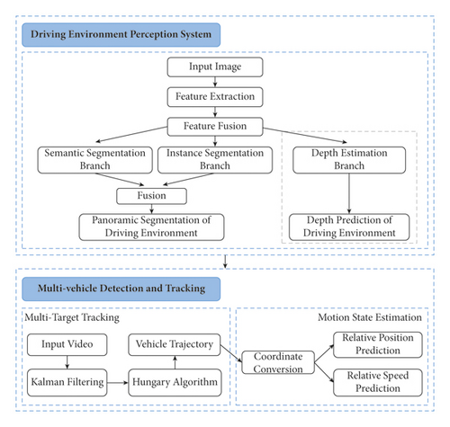
The methodology flowchart is presented in Figure 1. The methodology consists of two main parts: (1) a driving environment perception system and (2) multivehicle tracking and motion estimation. The driving environment perception system can realize the recognition and separation of vehicles and other elements in the driving environment through panoramic segmentation and then calculate the position of each vehicle by depth estimation. After obtaining the information of each vehicle at a time point, multivehicle tracking and state estimation is used to analyze the relationship between multiple vehicles in a continuous period of time. In the multivehicle tracking and state estimation method, vehicles between different frames in the video data are matched at first based on the segmentation results of the driving environment perception system. Then, the relative distance and relative speed between vehicles are estimated according to the depth information provided by the driving environment perception system. This kind of automatic calculation method of the relationship between multiple vehicles from camera videos can be used for advanced driver assistance systems to monitor the motions of vehicles and alter the potential collisions. These two parts are detailed below.

Details are in the caption following the image — **Figure 1**
Open in figure viewer PowerPoint

Methodology flowchart.

3.1. Driving Environment Perception Systems

The overall neural network structure of the environmental perception system mainly includes image feature extraction, feature fusion, semantic segmentation, instance segmentation, and depth estimation modules, as shown in Figure 2.

Step 1: feature extraction and fusion. Firstly, the input images go through the feature extraction module. The function of the feature extraction module is to extract the features of objects in the image, such as low-level features (e.g., edges and textures), as well as high-level features (e.g., skeletons and position relations among objects). Then, these features are input into the feature pyramid for fusion, and then these fused features serve as the basic input for semantic segmentation and instance segmentation.
Step 2: panoramic segmentation. Semantic segmentation is responsible for identifying the region class in the driving environment scene, while instance segmentation is used to support the instance class in the recognition scene. The output results of semantic segmentation and instance segmentation are fused to obtain the results of panoramic segmentation.
Step 3: depth estimation. Depth estimation branch and panorama segmentation share the features extracted by ResNet-FPN, and both of them require information about semantics, texture, and contour. In the depth estimation, pixels with the same semantics generally have similar depths, and the contours of each instance are the positions where the depth changes. Feature sharing avoids a separate step of feature extraction for depth estimation, which greatly reduces the amount of calculation.

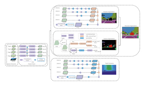
The panoramic segmentation and depth estimation in the network structure of this driving environment perception system are described in detail as follows.

3.1.1. Panoramic Segmentation of Driving Environment

The urban road driving environment is composed of road infrastructure, traffic signs and markings, and traffic participants. From the perspective of the panoramic segmentation task, the components of the driving environment of urban roads mainly include instance class and regional class. The regional class mainly contains pavement, greening, lane lines, guardrails, curbs, roadside buildings, and so forth, while the instance class includes signs, traffic lights, and traffic participants.

The feature extraction module uses the ResNet structure. ResNet can prevent network degradation so that the network can extract features with more neural layers. The overall structure of ResNet is formed by continuously stacking the bottleneck structure (BottleNeck). There are generally 4 stages, and the number of channels increases as the network depth increases. In general, the deeper the level, the smaller the size of the feature map and the more channels.

Feature pyramid network (FPN) uses a top-down network structure to integrate deep semantic features and simple detail features, which makes full use of the features extracted by the backbone network. The feature pyramid network is connected after the ResNet network and enriches the feature expression of the entire feature extraction network. FPN ensures that downstream tasks can obtain enough effective information to improve the accuracy of the model.

The network structure of the semantic segmentation branch adopts the ResNet-FPN network structure. The four output branches of ResNet-FPN, respectively, pass through their corresponding decoders to obtain a decoding result with a size of 1/4 of the original picture and 128 channels. The decoder consists of multiple convolution kernels with a size of 3 × 3 and 2 times upsampling. The number of the pairs of convolution and upsampling is determined according to the size of the input feature. The fusion of different branch predictions adopts the method of adding corresponding elements. The summation result is convolved to obtain the semantic prediction of the picture. The final predicted result is enlarged by 4 times to ensure the same size as the original image.

Instance segmentation is completed based on target detection. The task of target detection is to identify the object in the image, mark the position of the object, and determine its class. The segmentation branch network structure includes four parts: RPN, RoIAlign, R-CNN, and Mask. RPN (region proposal network) is the module responsible for generating candidate frames, and it finally provides Region of Interest (RoI) for downstream tasks. RoIAlign makes the features corresponding to RoI uniform in size. The Box branch predicts the class of each RoI and the correction coefficient of the box relative to the actual box. The Mask branch estimates the specific shape of the object in the box.

Finally, the prediction results of semantic segmentation and strength segmentation are merged to obtain panoramic segmentation results. Panorama segmentation requires that each pixel in the output prediction result can only be assigned a unique class and instance number. The overlap between instance objects is recognized as the object with high confidence. The part where instance segmentation and semantic segmentation overlap chooses the results of instance segmentation.

3.1.2. Depth Estimation of Driving Environment

Depth information under the urban road driving environment represents the distance information between the objects in the driving environment and the observation point. Depth estimation is to estimate the size of the distance value; namely, depth estimation refers to the depth of the pixel. According to the RGB information of the image, the distance between the object (corresponding to each pixel in the image) and the camera is estimated. Assuming that the input image is I and the image depth is D, the depth estimation task is to find a suitable function to map the image information into depth information, as shown in the following formula:

(1)

Depth estimation is similar to semantic segmentation, and both of them belong to pixel-by-pixel dense prediction tasks. Therefore, the branch of depth estimation can also use the Full Convolutional Network. The basic network structure of depth estimation is similar to the semantic segmentation branch. The input of the depth estimation branch is also the four output branches of the feature pyramid network. The size of each feature map is 1/32, 1/16, 1/8, and 1/4, respectively, and the number of channels is 256. Each branch is subjected to multiple convolutions and upsampling to obtain a tensor of size S and the number of channels C.

The number of convolution and upsampling operations is determined by the super parameter S. As shown in Figure 2, when S = 1/4, the depth estimation is conducted by 8 times of convolution and 7 times of upsampling. FPN-P1 (i.e., the first feature layer extracted by FPN) performs one convolution operation, FPN-P2 performs one pair of convolution and upsampling operations, FPN-P3 performs 2 pairs of convolution and upsampling operations, and FPN-P4 performs 3 pairs of convolution and upsampling operations. After these four output branches are added, a convolution operation and an upsampling operation are performed, and then the depth prediction value is obtained.

3.2. Multivehicle Tracking and Motion Estimation

3.2.1. Multitarget Tracking of Moving Vehicles

The main purpose of multitracking of moving vehicles is to obtain position and speed information of multiple vehicles. However, the difficulty of calculating the position and speed of moving vehicles mainly lies in the matching and tracking of objects between two different frames.

As for vehicle video data, the two frames of pictures are completely independent in encoding form. Therefore, the vehicles must be tracked between the two frames before the state of the vehicles can be calculated. The key to realizing multitarget vehicle trajectory tracking lies in the detection of vehicles in a single frame and the matching of objects between frames. For single-frame vehicle detection, the interframe detection frame is optimized by Kalman filtering according to the continuity of the video data. Then, the Hungarian matching algorithm is applied to match objects between frames.

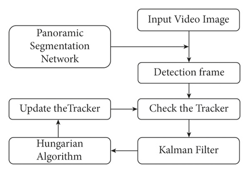
Specifically, the algorithm flow of vehicle trajectory multitarget tracking is as follows: Firstly, the image of each frame is continuously extracted from the video data and input into the panoramic segmentation network. The panoramic segmentation network in Figure 1 is used to detect the vehicle in the image and output the detection frame. Secondly, the status of the tracker is checked. Then, the Kalman filter is employed to estimate the optimal state of the detection frame. Besides, the Hungarian matching algorithm is used to match the tracking vehicles. Finally, if the tracker matches the detection frame successfully, update the tracker to a certain state. The flowchart of the tracking algorithm is shown in Figure 3.

Kalman filter is an optimal estimation algorithm that combines measurement data with the prediction model to achieve the optimal estimation of vehicle positions. Since the measurement data of vehicle positions are noisy, the measured value does not accurately reflect the true position of the car. Additionally, the noise of the prediction process is uncertain, so the prediction model cannot be solely used to estimate the vehicle positions. Thus, Kalman filters can provide a better estimation result by combining them to reduce the variance.

As shown in Figure 4, the working principle of the Kalman filter is explained intuitively by using the probability density functions. The predicted value of the vehicle position is near x_k, and the measured value of the vehicle position is near y_k. The variance represents the uncertainty of the estimation, and the actual position of the vehicle is different from the measured position and the predicted position. The best estimation of vehicle position is the combination of predicted and measured values. The best estimated probability density function is obtained by multiplying the two probability functions, and the variance of this estimate is less than the previous estimate. Therefore, Kalman filter can estimate the vehicle position in an optimized way.

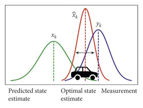
As shown in equation (2), the Kalman gain K refers to the ratio of the predicted error of the model to the measurement error of the panoramic segmentation detection system in the process of estimating the optimal state of the detection frame. K ∈ [0,1]. When K = 0, it indicates that the prediction error is 0, and the optimal state of the detection frame depends entirely on the predicted value of the model. When K = 1, it indicates that the observation error is 0, and the optimal condition of the detection frame entirely depends on the detection result of the panoramic segmentation system.

(2)

The principle of using the Kalman filter to estimate the optimal condition of the detection frame is to minimize the optimal estimation error covariance P_k. In this case, the estimated value is closer to the actual value.

The Hungarian algorithm [40] is a combinatorial optimization algorithm that solves the task assignment problem in polynomial time. The Hungarian algorithm is mainly used to solve some problems related to bipartite graph matching, and it is also used to solve the data association problem in multitarget tracking.

The matching of objects between frames is essentially a bipartite graph matching problem, so this paper uses the Hungarian algorithm to solve the problem of object matching between frames. Assuming that there are three trackers in the previous frame, the Kalman filter predicts that there are three vehicles in the current frame. In the current frame, three vehicles are detected by the detector. It is predicted that a certain car in the frame has the possibility to match each car in the detected frame. The Hungarian algorithm is to find the best match between the predicted frame and the detected frame, as shown in Figure 5. Each prediction frame and each detection frame have a cost (unreliability), and then prediction frames and detection frames form a cost matrix. The Hungarian algorithm obtains the matching result between the two frames by transformation and calculation of the cost matrix.

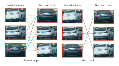
The definition of the cost matrix will directly affect the quality of the matching result. From the perspective of the position of the detection frame, since the time between frames is short and the moving speed of the vehicle is limited, the detection frame of the same object between the two frames should be relatively close. From the perspective of the appearance of the object, it has similar characteristics for the same object. Therefore, the setting of the cost matrix will be considered from the two perspectives of distance and feature difference.

Since the Hungarian algorithm belongs to the maximum matching algorithm, matching will be completed to the greatest extent. There are constantly vehicles leaving the camera’s perspective in the scene; meanwhile, new vehicles are entering the camera’s perspective. To improve the matching accuracy, a screening based on Mahalanobis distance and appearance distance is performed on the matching results. When the Mahalanobis distance and the appearance distance of a certain match between two corresponding detection frames are less than a certain threshold, the matching is accepted; otherwise the matching is abandoned.

3.2.2. Multivehicle Motion Estimation

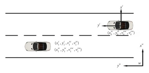
The position and speed of the moving vehicle in the driving environment can be divided into lateral and longitudinal according to different directions, that is, lateral distance, longitudinal distance, lateral speed, and longitudinal speed. In different coordinate systems, the way of expression is different. As shown in Figure 6(a), there are the world coordinate system x^wwy^w and the camera coordinate system x^ccy^c. The position state of the origin of the camera coordinate system in the world coordinate system is , and the speed state is . is the velocity component of the camera coordinate system in the x direction of the world coordinate system, and is the velocity component of the camera coordinate system in the y direction of the world coordinate system. The states of vehicles in different coordinates can be converted mutually. The state of the vehicle in the world coordinate system is the vector sum of the state of the camera in the world coordinate system and the state of the vehicle in the camera coordinate system .

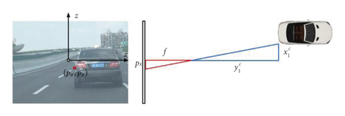
The distance calculation includes the lateral distance and the longitudinal distance. For the estimation of the longitudinal distance, the depth information can be obtained from the depth estimation network in Methodology section above. For the calculation of the lateral distance, it can be estimated through its geometric relationship with the longitudinal distance.

As shown in Figure 6(b), the coordinates of the vehicle in front of the camera in the camera coordinate system are

. The vehicle is imaged in the camera, and the coordinates in the picture coordinate system xoz are (p_x, p_z). The two triangles formed by light are similar, which can be derived from the properties of similar triangles:

(3)

where f is the focal length of the camera.

To calculate the vehicle speed, it first needs to determine the changes in the lateral and longitudinal distances

of the object in the two adjacent frames of images recorded by the camera coordinate system. Then, according to the relationship between displacement and speed, the lateral and vertical speed of the object in the camera coordinate system can be obtained.

(4)

where Δt is the time difference between two frames, which is the reciprocal of the number of frames per second recorded by the camera.

By calculating the relative lateral and vertical distances and relative lateral and vertical speeds between vehicles, the motion state of multiple vehicles can be estimated so that the relative relationship between multiple vehicles can be further studied.

In conclusion, using the multitarget tracking algorithm, vehicle detection is optimized, and the problem of vehicle matching between frames is solved. Through the depth information and coordinate conversion method, the position and speed of the moving vehicle can be estimated, so that the relative relationship between multiple vehicles is obtained.

4. Model Training and Case Study

4.1. Driving Environment Perception Experiment

4.1.1. Panoramic Segmentation Experiment of Driving Environment

The dataset used for the training is the Mapillary Vistas Dataset (MVD) [41]. MVD is a novel, large-scale, street-level image dataset containing 25000 high-resolution images, with an average number of 8.6 million pixels per image. Training and validation data comprise 18000 and 2000 images, respectively, and the remaining 5000 images form the test set.

The loss of the whole panoramic segmentation network consists of two parts, namely, semantic segmentation loss and instance segmentation loss. The loss of panoramic segmentation is

(5)

where λ is the loss adjustment factor between two subpartition missions.

Semantic segmentation loss y = {1, …, N_classes}is the class set of semantic prediction, Y_ij ∈ y is the actual class of pixels of a given image at (i, j), and P_i,j(c) is the probability value of pixels of an image at (i, j) belonging to class C. The loss of semantic segmentation for a single image is calculated according to the following equation:

(6)

Instance Segmentation Loss. The loss of the instance segmentation consists of three parts: the RPN, the Box, and the Mask. Therefore, the loss of instance segmentation is

(7)

The Calculation of the Loss of the RPN. The loss of judging whether there is an object in the bounding box is

, and the loss of the position of the bounding box is

. The sample pair M^± contains both a positive sample pair M₊ and a negative sample pair M₋. r is the actual bounding box r = (x_r, y_r, w_r, h_r), and

is the predicted bounding box

is the probability that an object is contained in

predicted in RPN.

refers to the default frame, and |·|_S refers to smooth loss.

(8)

The Calculation of the Loss of the Box Branch. The loss of Box class prediction is

, and the loss of the position of the bounding box is

. The sample pair N contains the positive sample pair set N₊ and the negative sample pair set N₋. c_r is the class corresponding to the actual bounding box r, and

is the probability that the predicted box belongs to class c.

(9)

The Calculation of the Loss of the Mask Branch. S^r is the binary mask corresponding to object c in the bounding box r,

is the binary mask of class c predicted by the Mask branch, and

is the probability that cell(i, j) belongs to class c. d is the side length of the mask, which is 28.

(10)

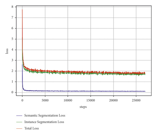
The overall loss of the training process is shown in Figure 7. As shown in Figure 7, the loss value keeps decreasing and tends to be stable with the progress of training, indicating that the training results converge, the network design is reasonable, and the training strategy is correct.

The trained model is used to predict the image of the MVD validation set, and the accuracy of the model is calculated according to the evaluation indexes (RQ (recognition quality), SQ (segmentation quality), and PQ (panoptic quality); PQ = RQ × SQ) [42] of panoramic segmentation, as shown in Table 1. The PQ value of the validation set reached 15.224%. Compared with the results of some other methods in previous studies [43], the recognition effect in this study was good.

Table 1. Panoramic segmentation accuracy.

	PQ (%)	SQ (%)	RQ (%)
All	15.224	34.267	19.008
Things	10.219	29.021	13.136
Stuff	21.837	41.198	26.767
Reference value (all) 43	11.465–16.931	28.624–35.857	13.041–22.163

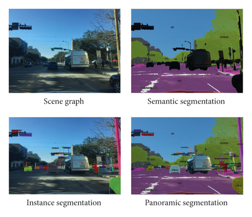
The visualization of the prediction results is shown in Figure 8. Figure 8(a) shows the result of the semantic segmentation branch, which accurately divides the road, sidewalk, greening, building, and sky. Figure 8(c) shows the detection and segmentation effect of the instance segmentation branch, which accurately detects and divides vehicles, pedestrians, traffic lights, and pillars. Figure 8(d) is the result of semantic segmentation and instance segmentation fusion.

4.1.2. Depth Estimation Experiment of Driving Environment

The dataset used for training the depth estimation algorithm is the Cityscapes Depth Dataset [44]. The Cityscapes Depth Dataset collects binocular pictures with binocular cameras and is calculated by the SGM algorithm [45]. The scene includes a total of 5,000 pictures of urban roads in different seasons of multiple cities in Europe, including 2,975 in the training set, 500 in the validation set, and 1,525 in the test set.

The loss function uses berHu [46] loss function, and the calculation formula is

(11)

where

is the depth prediction value of pixel i; d_i is the actual depth value of pixel i; N is the total number of picture pixels;

The weights of the ResNet-FPN and panorama segmentation parts of the model remain unchanged, and only the weights of the depth estimation branch are trained and updated. The optimization algorithm for model training uses the stochastic gradient descent algorithm, in which the momentum parameter is set to 0.9 and the weight attenuation coefficient is set to 0.0001. The basic learning rate is set to 0.001, the number of optimization iterations of the model is 20000, and the batch size of the optimized image is 4 for each iteration. The feature map size of the depth estimation branch structure parameter S is 1/4, and the feature map channel number C is equal to 128.

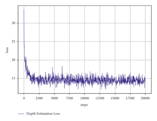
The loss change of the depth estimation during the training process is shown in Figure 9. The loss drops rapidly in the first 2000 rounds of training and then basically stabilizes after 5000 rounds of iterations.

The trained model is used to predict the images in the verification set of the Cityscapes Depth Dataset. According to the evaluation index of the depth estimation, the accuracy of the calculated model is shown in Table 2. The evaluation indicators used in the depth estimation include relative error (rel), root mean square error (rms), root mean square error in logarithmic space (rms_log), and accuracy (P) under different thresholds (i.e., accuracy threshold is 1.25, 1.25², 1.25³). It can be seen that the number of pixels with a deviation ratio between the predicted value and the true value within 1.25, 1.25², and 1.25³ accounted for 63.6%, 81.7%, and 90.5%, respectively. Compared with the similar method in current studies [47], this method used in our study has a good performance.

Table 2. Depth estimation accuracy.

Evaluation index	P_1.25			rel	rms	rms_log
Result	63.6%	81.7%	90.5%	0.276	35.198	0.116
Reference value [47]	50.8%–65.0%	75.5%–83.4%	82.7%–91.2%	0.169–0.308	25.652–37.231	0.103–0.119
Explanation	Higher is better			Lower is better

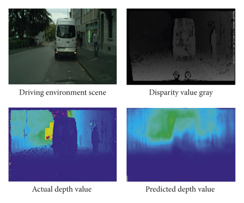
Figures 10(b) and 10(c) are visualization diagrams of the actual and predicted depth values, respectively. The overall trend of depth prediction is generally correct. From near to far, the color deepens, and the depth value gradually increases. From a local perspective, the depth prediction successfully captures the location and range of vehicles and pedestrians. Their depth is smaller than the surroundings, and there is a sudden change in the depth value of the outline.

4.2. Motion Estimation of Multiple Vehicles

4.2.1. Traffic Simulation Test Design

Evaluating the accuracy of the state estimation of the multitarget moving vehicles requires the real state of the vehicles in front as a comparison. The real motion state data of the preceding vehicle is obtained through the traffic simulation experiment that uses the traffic simulation software SiLab, multiperson driving traffic simulation software. Not only is the scene highly reproducible, but also each car is controlled by a driver with certain driving experience, which simulates the real traffic driving environment to the greatest extent. SiLab can record and output the position and movement information of each vehicle in real time. The recorded data used in subsequent calculations of this experiment are mainly timestamps, X-axis and Y-axis coordinates, and speed of the vehicle. The simulated driving system uses the Logitech G29 simulator control package, which includes a steering wheel, pedals, and shifters. The entire multiperson driving platform is equipped with 1 main driving position and 4 ordinary driving positions, and up to 5 people can drive at the same time, as shown in Figure 11(a).

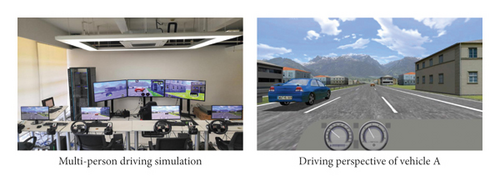
The simulated driving scene is set to one-way three lanes, as shown in Figure 11(b). The specific experimental plan is to run three cars (denoted as A, B, and C) on the multiperson driving platform SiLab at the same time. The driving perspective of vehicle A is regarded as the camera perspective, and vehicles B and C are treated as the observation objects.

In the simulated driving experiment, the common vehicle speed on urban roads is used, ranging from 60 km/h to 80 km/h. The movement speed will affect the recognition and tracking accuracy of multitarget tracking [48]. When the vehicle speed is slower, the effect of maintaining the detection result is stable. When the vehicle speed is faster, the detection result may appear to be fluctuant. The simulation driving experiment results show that the detection accuracy of multitarget tracking is about 86.3% when the vehicle speed is in the range of 40 km/h to 60 km/h; the detection precision is about 75.8% when the vehicle speed is in the range of 60 km/h to 80 km/h.

4.2.2. Moving Vehicle Distance and Speed Estimation

The sampling frequency of vehicle motion state data is set to 60 Hz in SiLab, and the frequency of driving perspective recording is also equal to 60 Hz. In this way, each frame of the driving perspective corresponds to a piece of data in SiLab. The format of vehicle A’s motion state data from the SiLab output is shown in Table 3.

Table 3. Panoramic segmentation accuracy.

Measurement time (ms)	Y (m)	X (m)
66.68	19.984300	7.125050
83.34	19.984300	7.125050
100.01	19.984300	7.125050
116.67	19.984300	7.125050
133.34	19.984300	7.125050

According to the lateral and longitudinal movement distances between two different moments, the lateral and longitudinal speeds of cars A, B, and C are calculated. According to equations (12) and (13), the coordinates of cars B and C in the camera coordinate system centered on car A are calculated. According to equations (14) and (15), the lateral and longitudinal relative speeds of cars B and C with car A as the reference system are calculated.

(12)

(13)

(14)

(15)

The above algorithm is implemented in the Python software. The video of the driving perspective of car A is processed, and the motion states of car B are estimated, as demonstrated in Table 4.

Table 4. Motion state prediction.

Frame number	Tracker number	x^c (m)	y^c (m)	v^xc (m/s)	v^yc (m/s)
7383	95	5.1	10.1	0.5	0.9
7384	95	5.1	10.1	0.0	0.0
7385	95	5.1	10.1	0.0	0.0
7386	95	3.9	9.5	−1.2	0.0

As illustrated in Figure 12, taking vehicle B as an example, with vehicle A as the camera perspective, the relative position and relative speed of vehicle B are predicted and compared with the actual state of motion.

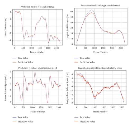
The estimation results of the algorithm proposed in this study on the lateral relative distance of moving vehicles are shown in Figure 12(a). The estimated value of the algorithm is consistent with the actual value. From a quantitative perspective, the average error of the lateral relative distance is 0.186 m, and the average relative error is 11.5%. The estimation of the longitudinal relative distance of the moving vehicle is shown in Figure 12(b). The algorithm has better accuracy for estimating the distance within 50 meters, and there is a large error in the estimation of the distance beyond 50 meters. The reason for the larger error is related to the characteristics of monocular visual depth estimation. There is less information in the distance, the larger the error is. From a quantitative perspective, the average error of the longitudinal relative distance is 1.86 m, and the average relative error is 7.0%.

The estimation of the lateral relative speed of moving vehicles is shown in Figure 12. Thanks to the small lateral relative distance error, the estimated value of the lateral relative speed is consistent with the actual value. The average error of the lateral relative velocity is 0.186 m/s, and the average relative error is 1.5%. The estimation results of the longitudinal relative speed of the moving vehicle are shown in Figure 12(d). The estimated value of the algorithm is similar to the actual value, and there is a certain fluctuation. After calculation, the average error of the longitudinal relative velocity is 0.37 m/s, and the average relative error is 5.0%.

In general, experiments have proved that the vehicle multitarget tracking algorithm in this study is feasible and has good performance with high accuracy in the estimation of distance and speed.

5. Conclusion

The perception of the driving environment on urban roads and the realization of vehicle tracking and motion state estimation are the indispensable parts of assisted driving and autonomous driving. This study proposes a novel multitarget vehicle tracking and motion state estimation method based on a new driving environment perception system. Compared with the previous research on multitarget vehicle tracking, the driving environment perception system developed in this study can obtain rich driving environment information without interference between vehicles. The driving environment perception system establishes a lightweight neural network and adds depth estimation based on panoramic segmentation to estimate the state of vehicle motion and explore the relationship between multiple vehicles.

Firstly, a neural network that supports end-to-end training is designed and implemented. The network features are extracted by ResNet. The features are integrated by the feature pyramid as the input of semantic segmentation branch and instance segmentation, and the segmentation output of the two branches is merged to obtain the result of panoramic segmentation. After training and prediction on the MVD, the PQ value of the validation set reached 15.22. The final model has reached a high level in terms of accuracy and visual effects. The depth estimation branch is designed to realize the monocular range of the road scene. Through training and prediction on the Cityscapes Depth Dataset, the relative error on the validation set is 0.276, and it is proved that the model can achieve good accuracy in the depth estimation of monocular vision.

Secondly, based on the recognition result of the driving environment realized by the panoramic segmentation, the Kalman filter and the Hungarian algorithm are used to realize the multitarget tracking of the vehicle. Combining the distance information obtained by depth estimation, the relative speed of the vehicle is estimated. The multitarget tracking algorithm is used to solve the matching problem of state calculation. The results of the simulated driving test show the following: (1) The average error of the lateral relative distance is 0.19 m, and the longitudinal direction is 1.86 m. (2) The average error of the lateral relative velocity is 0.19 m/s, and the longitudinal direction is 0.37 m/s. This simulation experiment proves that the algorithm performs well in multitarget tracking.

The findings of this study can contribute to the development of intelligent vehicles to alert drivers to possible danger, assist drivers’ decision-making, and improve traffic safety. To be specific, this study can be used to identify roads and lane markings and warn drivers of lane departure. When the vehicle approaches the lane markings, the driver is reminded in the form of sound or image [49]. The multivehicle tracking and motion estimation in this study can be used in an adaptive cruise control system. According to the relative speed and distance to the front vehicle, it adaptively controls its own brakes and accelerators to maintain a certain distance and similar speed with the front vehicle. In the actual driving environment, a digital platform can be established to interact with the driver through the driving environment perception system. Through the driving recorder to obtain pictures or videos of other vehicles, the digital platform calculates the position information of multiple vehicles in real time and displays the trajectories of multiple vehicles over time to the driver.

The deep neural network framework proposed in this study is highly shared in computing, and task branches can be added or deleted conveniently according to actual needs. Multitarget vehicle tracking through image segmentation only relies on easily available data such as images and videos, and the equipment is convenient to install and simple to use. However, due to the use of monocular vision for distance measurement in the depth estimation, there is a problem of limited accuracy in estimating the vehicle’s motion state. In the future, we will try to use binocular distance measurement for depth estimation to obtain more accurate motion status information for multiple vehicles.

Conflicts of Interest

The authors declare that there are no conflicts of interest regarding the submission of this manuscript.

Acknowledgments

This project was supported by the National Key Research and Development Program of China (no. 2017YFC0803902), the Fundamental Research Funds for the Central University (no. 22120210431), and the National Natural Science Foundation of China (no. 52102416).

Open Research

Data Availability

The data used to support the findings of this study are available from the corresponding author upon request.

References

1 Dingus T. A., Klauer S. G., Neale V. L., Perez M. A., Sudweeks J., Peterson A., and Lee E. S., The 100-car naturalistic driving study, phase II—results of the 100-car field experiment, National Highway Traffic Safety Administration. (2006) .
Google Scholar
2 National Bureau of Statistics, Statistics on the causes of traffic accidents, “Traffic accident data”, 2021, National Bureau of Statistics, http://wap.stats.gov.cn.
Google Scholar
3 Wang F. Y., Mirchandani P. B., and Wang Z., The VISTA project and its applications, IEEE Intelligent Transportation Systems. (2002) 17, 1134364, https://doi.org/10.1109/mis.2002.1134364, 2-s2.0-0141837102.
10.1109/mis.2002.1134364
Google Scholar
4 Yu B., Bao S., Feng F., and Sayer J., Examination and prediction of drivers’ reaction when provided with V2I communication-based intersection maneuver strategies, Transportation Research Part C: Emerging Technologies. (2019) 106, 17–28, https://doi.org/10.1016/j.trc.2019.07.007, 2-s2.0-85068898756.
10.1016/j.trc.2019.07.007
Web of Science® Google Scholar
5 Yu B., Bao S., Zhang Y., Sullivan J., and Flannagan M., Measurement and prediction of driver trust in automated vehicle technologies: an application of hand position transition probability matrix, Transportation Research Part C: Emerging Technologies. (2021) 124, https://doi.org/10.1016/j.trc.2020.102957.
10.1016/j.trc.2020.102957
Web of Science® Google Scholar
6 Wang K., Li Z., Sun Y., Wang F., and Qiao X., An embedded system for vision-based driving environment perception, Proceedings of the 2006 2nd IEEE/ASME International Conference on Mechatronics and Embedded Systems and Applications, August 2006, Beijing, China, https://doi.org/10.1109/mesa.2006.296998, 2-s2.0-44949202718.
10.1109/mesa.2006.296998
Google Scholar
7 Yu B., Chen Y., and Bao S., Quantifying visual road environment to establish a speeding prediction model: an examination using naturalistic driving data, Accident Analysis & Prevention. (2019) 129, 289–298, https://doi.org/10.1016/j.aap.2019.05.011, 2-s2.0-85066799870.
10.1016/j.aap.2019.05.011
PubMed Web of Science® Google Scholar
8 Yu B., Chen Y., Bao S., and Xu D., Quantifying drivers′ visual perception to analyze accident-prone locations on two-lane mountain highways, Accident Analysis & Prevention. (2018) 119, 122–130, https://doi.org/10.1016/j.aap.2018.07.014, 2-s2.0-85049830655.
10.1016/j.aap.2018.07.014
PubMed Web of Science® Google Scholar
9 Li Y., Zhang Y., Shi H. et al., Visual analytic method for metro anomaly detection and diffusion, Journal of Advanced Transportation. (2020) 2020, 12, 9082370, https://doi.org/10.1155/2020/9082370.
10.1155/2020/9082370
Web of Science® Google Scholar
10 Liu Z. Q., Zhang T., and Wang Y. F., Research on local dynamic path planning method for intelligent vehicle lane-changing, Journal of Advanced Transportation. (2019) 2019, 10, 4762658, https://doi.org/10.1155/2019/4762658, 2-s2.0-85064347831.
10.1155/2019/4762658
Google Scholar
11 Zhang K., Ren H., Wei Y., and Gong J., Multi-target vehicle detection and tracking based on video, Proceedings of the 32nd China Control and Decision Making Conference, August 2020, Hefei, China, https://doi.org/10.1109/ccdc49329.2020.9164621.
10.1109/ccdc49329.2020.9164621
Google Scholar
12 Lin S., Tang J., Zhang X., and Lv Y., Research on traffic moving object detection, tracking and track-generating, Proceedings of the 2009 IEEE International Conference on Automation and Logistics, 2009, Shanyang, China, IEEE, https://doi.org/10.1109/ical.2009.5262818, 2-s2.0-70450169066.
10.1109/ical.2009.5262818
Google Scholar
13 Redmon J., Divvala S., Girshick R., and Farhadi A., You only look once: unified, real-time object detection, Proceedings of the IEEE Conference on Computer Vision and Pattern Recognition, June 2016, Las Vegas, NV, USA, https://doi.org/10.1109/cvpr.2016.91, 2-s2.0-84986308404.
10.1109/cvpr.2016.91
Google Scholar
14 Redmon J. and Farhadi A., YOLO9000: better, faster, stronger, Proceedings of IEEE Conference on Computer Vision & Pattern Recognition, June 2017, Honolulu, HI, USA, 6517–6525, https://doi.org/10.1109/cvpr.2017.690, 2-s2.0-85041900441.
10.1109/cvpr.2017.690
Google Scholar
15 Guo Y., Sayed T., and Essa M., Real-time conflict-based Bayesian Tobit models for safety evaluation of signalized intersections, Accident Analysis & Prevention. (2020) 144, 105660, https://doi.org/10.1016/j.aap.2020.105660.
10.1016/j.aap.2020.105660
PubMed Web of Science® Google Scholar
16 Wu W., Kozitsky V., Hoover M. E., Todd Jackson M. D., and Loce R. P., Vehicle speed estimation using a monocular camera, Video Surveillance and Transportation Imaging Applications. (2015) https://doi.org/10.1117/12.2083394, 2-s2.0-84925014478.
10.1117/12.2083394
Google Scholar
17 Liang Y., Research on Front Vehicle Detection Method Based on Millimeter-Wave Radar and Deep Learning Visual Information Fusion, 2019, South China University of Technology, China.
Google Scholar
18 Li C., Motion Perception and Lane-Changing Intention Recognition of the Vehicle in Front of the Smart Car, 2019, Xi'an University of Technology, Xian, China.
Google Scholar
19 Chen X., Li Z., Yang Y., Qi L., and Ke R., High-resolution vehicle trajectory extraction and denoising from aerial videos, IEEE Transactions on Intelligent Transportation Systems. (2021) 22, no. 5, 3190–3202, https://doi.org/10.1109/tits.2020.3003782.
10.1109/TITS.2020.3003782
Web of Science® Google Scholar
20 Chen X., Lu J., Zhao J., Qu Z., Yang Y., and Xian J., Traffic flow prediction at varied time scales via ensemble empirical mode decomposition and artificial neural network, Sustainability. (2020) 12, no. 9, https://doi.org/10.3390/su12093678.
10.3390/su12093678
Web of Science® Google Scholar
21 Tu Z., Chen X., Yuille A. L., and Zhu S.-C., Image parsing: unifying segmentation, detection, and recognition, International Journal of Computer Vision. (2005) 63, no. 2, 113–140, https://doi.org/10.1007/s11263-005-6642-x, 2-s2.0-17444392134.
10.1007/s11263-005-6642-x
Web of Science® Google Scholar
22 Li Q., Arnab A., and Torr P. H., Weakly-and semi-supervised panoptic segmentation, Proceedings of the European Conference on Computer Vision (ECCV), September 2018, Munich, Germany, 102–118, https://doi.org/10.1007/978-3-030-01267-0_7, 2-s2.0-85055433314.
10.1007/978-3-030-01267-0_7
Google Scholar
23 Scharstein D. and Szeliski R., A taxonomy and evaluation of dense two-frame stereo correspondence algorithms, International Journal of Computer Vision. (2002) 47, no. 1/3, 7–42, https://doi.org/10.1023/a:1014573219977, 2-s2.0-0036537472.
10.1023/A:1014573219977
Web of Science® Google Scholar
24 Forsyth D. and Ponce J., Computer Vision: A Modern Approach, 2002, Prentice-Hall Professional Technical Reference, New Jersey, NJ, USA.
Google Scholar
25 Saxena A., Chung S. H., and Ng A. Y., Learning depth from single monocular images, Advances in Neural Information Processing Systems. (2006) 1161–1168.
Google Scholar
26 Saxena A., Sun M., and Ng A. Y., Make3d: learning 3d scene structure from a single still image, IEEE Transactions on Pattern Analysis and Machine Intelligence. (2008) 31, 824–840.
10.1109/TPAMI.2008.132
Web of Science® Google Scholar
27 Hoiem D., Efros A. A., and Hebert M., Recovering surface layout from an image, International Journal of Computer Vision. (2007) 75, no. 1, 151–172, https://doi.org/10.1007/s11263-006-0031-y, 2-s2.0-34547216923.
10.1007/s11263-006-0031-y
Web of Science® Google Scholar
28 Ladicky L., Shi J., and Pollefeys M., Pulling things out of perspective, Proceedings of the IEEE Conference on Computer Vision and Pattern Recognition, June 2014, Columbus, OH, USA, 89–96, https://doi.org/10.1109/cvpr.2014.19, 2-s2.0-84911412663.
10.1109/cvpr.2014.19
Google Scholar
29 Li X., Qin H., Wang Y., and Zhang Y., Dept: depth estimation by parameter transfer for single still images, Proceedings of the Asian Conference on Computer Vision, November 2014, Singapore, 45–58.
Google Scholar
30 Choi S., Min D., Ham B., Kim Y., Oh C., and Sohn K., Depth analogy: data-driven approach for single image depth estimation using gradient samples, IEEE Transactions on Image Processing. (2015) 24, no. 12, 5953–5966, https://doi.org/10.1109/tip.2015.2495261, 2-s2.0-84960193272.
10.1109/TIP.2015.2495261
PubMed Web of Science® Google Scholar
31 Liu M., Salzmann M., and He X., Discrete-continuous depth estimation from a single image, Proceedings of the IEEE Conference on Computer Vision and Pattern Recognition, June 2014, Columbus, OH, USA, 716–723, https://doi.org/10.1109/cvpr.2014.97, 2-s2.0-84911384005.
10.1109/cvpr.2014.97
Google Scholar
32 Zhuo W., Salzmann M., He X., and Liu M., Indoor scene structure analysis for single image depth estimation, Proceedings of the IEEE Conference on Computer Vision and Pattern Recognition, June 2015, Boston, MA, USA, 614–622, https://doi.org/10.1109/cvpr.2015.7298660, 2-s2.0-84959245228.
10.1109/cvpr.2015.7298660
Google Scholar
33 Simonyan K. and Zisserman A., Very deep convolutional networks for large-scale image recognition, 2014, https://arxiv.org/abs/1409.1556.
Google Scholar
34 Szegedy C., Liu W., Jia Y., Erhan D., and Reed S., Going deeper with convolutions, Proceedings of the IEEE Conference on Computer Vision and Pattern Recognition, June 2015, Boston, MA, USA, 1–9, https://doi.org/10.1109/cvpr.2015.7298594, 2-s2.0-84937522268.
10.1109/cvpr.2015.7298594
Google Scholar
35 He K., Zhang X., and Ren S., Deep residual learning for image recognition, Proceedings of the IEEE Conference on Computer Vision and Pattern Recognition, June 2016, Las Vegas, NV, USA, 770–778, https://doi.org/10.1109/cvpr.2016.90, 2-s2.0-84986274465.
10.1109/cvpr.2016.90
Google Scholar
36 Eigen D., Puhrsch C., and Fergus R., Depth map prediction from a single image using a multi-scale deep network, Advances in Neural Information Processing Systems. (2014) 2366–2374.
Google Scholar
37 Xie J., Girshick R., and Farhadi A., Deep3d: fully automatic 2d-to-3d video conversion with deep convolutional neural networks, Proceedings of the European Conference on Computer Vision - ECCV 2016, October 2016, Armsterdam, Netherlands, 842–857, https://doi.org/10.1007/978-3-319-46493-0_51, 2-s2.0-84990046450.
10.1007/978-3-319-46493-0_51
Google Scholar
38 Garg R., B.G. V. K., Carneiro G., and Reid I., Unsupervised CNN for single view depth estimation: geometry to the rescue, Proceedings of the European Conference on Computer Vision - ECCV 2016, October 2016, Armsterdam, Netherlands, 740–756, https://doi.org/10.1007/978-3-319-46484-8_45, 2-s2.0-84990026532.
10.1007/978-3-319-46484-8_45
Google Scholar
39 Kuznetsov Y., Stuckler J., and Leibe B., Semi-supervised deep learning for monocular depth map prediction, Proceedings of the IEEE Conference on Computer Vision and Pattern Recognition, June 2017, Honolulu, HI, USA, 6647–6655.
Google Scholar
40 Kuhn H. W., The Hungarian method for the assignment problem, Naval Research Logistics Quarterly. (1955) 2, no. 1-2, 83–97, https://doi.org/10.1002/nav.3800020109.
10.1002/nav.3800020109
Google Scholar
41 Neuhold G., Ollmann T., and Bulo S. R., The mapillary vistas dataset for semantic understanding of street scenes, Proceedings of the IEEE International Conference on Computer Vision, October 2017, Venice, Italy, 4990–4999, https://doi.org/10.1109/iccv.2017.534, 2-s2.0-85034013319.
10.1109/iccv.2017.534
Google Scholar
42 Kirillov A., He K., and Girshick R., Panoptic segmentation, Proceedings of the IEEE Conference on Computer Vision and Pattern Recognition, June 2019, Long Beach, CA, USA, 9404–9413, https://doi.org/10.1109/cvpr.2019.00963.
10.1109/cvpr.2019.00963
Google Scholar
43 Tychsen-Smith L. and Petersson L., Denet: scalable real-time object detection with directed sparse sampling, Proceedings of the IEEE International Conference on Computer Vision, October 2017, Venice, Italy, 428–436, https://doi.org/10.1109/iccv.2017.54, 2-s2.0-85041921990.
10.1109/iccv.2017.54
Google Scholar
44 Cordts M., Omran M., and Ramos S., The cityscapes dataset for semantic urban scene understanding, Proceedings of the IEEE Conference on Computer Vision and Pattern Recognition, June 2016, Las Vegas, NV, USA, 3213–3223, https://doi.org/10.1109/cvpr.2016.350, 2-s2.0-84986255616.
10.1109/cvpr.2016.350
Google Scholar
45 Hirschmuller H., Accurate and efficient stereo processing by semi-global matching and mutual information, 2, Proceedings of the 2005 IEEE Computer Society Conference on Computer Vision and Pattern Recognition (CVPR’05), June 2005, San Diego, CA, USA, 807–814.
Google Scholar
46 Laina I., Rupprecht C., and Belagiannis V., Deeper depth prediction with fully convolutional residual networks, Proceedings of the 2016 Fourth International Conference on 3D Vision (3DV), October 2016, Stanford, CA, USA, 239–248, https://doi.org/10.1109/3dv.2016.32, 2-s2.0-85011317214.
10.1109/3dv.2016.32
Google Scholar
47 Zhao C., Sun Q., Zhang C., Tang Y., and Qian F., Monocular depth estimation based on deep learning: an overview, Science China Technological Sciences. (2020) 63, no. 9, 1612–1627, https://doi.org/10.1007/s11431-020-1582-8.
10.1007/s11431-020-1582-8
Web of Science® Google Scholar
48 Wojke N., Bewley A., and Paulus D., Simple online and realtime tracking with a deep association metric, Proceedings of the 2017 IEEE International Conference on Image Processing (ICIP), September 2017, Beijing, China, IEEE, 3645–3649, https://doi.org/10.1109/icip.2017.8296962, 2-s2.0-85045318361.
10.1109/icip.2017.8296962
Google Scholar
49 Luo Q., Chen X., and Yuan J., Study and simulation analysis of vehicle rear-end collision model considering driver types, Journal of Advanced Transportation. (2020) https://doi.org/10.1155/2020/7878656.
10.1155/2020/7878656
Web of Science® Google Scholar

Citing Literature

All articles

Multitarget Vehicle Tracking and Motion State Estimation Using a Novel Driving Environment Perception System of Intelligent Vehicles

Abstract

1. Introduction