Volume 2021, Issue 1 6221545

Research Article

Open Access

Bearing Faulty Prognostic Approach Based on Multiscale Feature Extraction and Attention Learning Mechanism

Corresponding Author

Yiqing Zhou

[email protected]

orcid.org/0000-0002-5633-9287

Computer Integrated Manufacturing System (CIMS) Research Center, College of Electronics and Information Engineering, Tongji University, Shanghai 201804, China tongji.edu.cn

Search for more papers by this author

Jian Wang,

Jian Wang

Computer Integrated Manufacturing System (CIMS) Research Center, College of Electronics and Information Engineering, Tongji University, Shanghai 201804, China tongji.edu.cn

Search for more papers by this author

Zeru Wang,

Zeru Wang

CAD Research Center, College of Electronics and Information Engineering, Tongji University, Shanghai 201804, China tongji.edu.cn

Search for more papers by this author

Yiqing Zhou,

Corresponding Author

Yiqing Zhou

[email protected]

orcid.org/0000-0002-5633-9287

Computer Integrated Manufacturing System (CIMS) Research Center, College of Electronics and Information Engineering, Tongji University, Shanghai 201804, China tongji.edu.cn

Search for more papers by this author

Jian Wang,

Jian Wang

Computer Integrated Manufacturing System (CIMS) Research Center, College of Electronics and Information Engineering, Tongji University, Shanghai 201804, China tongji.edu.cn

Search for more papers by this author

Zeru Wang,

Zeru Wang

CAD Research Center, College of Electronics and Information Engineering, Tongji University, Shanghai 201804, China tongji.edu.cn

Search for more papers by this author

First published: 22 November 2021

https://doi.org/10.1155/2021/6221545

Citations: 1

Academic Editor: Kelvin Wong

Share a link

Email
Wechat
Bluesky

Abstract

Recently, researches on data-driven faulty identification have been achieving increasing attention due to the fast development of the modern conditional monitoring technology and the availability of the massive historical storage data. However, most industrial equipment is working under variable industrial operating conditions which can be a great challenge to the generalization ability of the normal data-driven model trained by the historical storage operating data whose distribution might be different from the current operating datasets. Moreover, the traditional data-driven faulty prognostic model trained on massive historical data can hardly meet the real-time requirement of the practical industry. Since the hierarchical feature extraction can enhance the model generalization ability and the attention learning mechanism can promote the prediction efficiency, this paper proposes a novel bearing faulty prognostic approach combining the U-net-based multiscale feature extraction network and the CBAM- (convolutional block attention module-) based attention learning network. First, time domain conditional monitoring signals are converted into the two-dimensional gray-scale image which can be applicable for the input of the CNN. Second, a CNN model based on the U-net structure is adopted as the feature extractor to hierarchically extract the multilevel features which can be very sensitive to the faulty information contained in the converted image. Finally, the extracted multilevel features containing different representations of the raw signals are sent to the designed CBAM-based attention learning network for high efficiency faulty classification with its unique emphasize discrimination characteristic. The effectiveness of the proposed approach is validated by two case studies offered by the CWRU (Case Western Reserved University) and the Paderborn University. The experimental result indicates that the proposed faulty prognostic approach outperforms other comparison models in terms of the generalization ability and the speed-up properties.

1. Introduction

With the advent of the large-scale manufacturing of the modern industry, the prognostic and health management (PHM) of the manufacturing equipment has been becoming increasingly important. Bearings, regarded as the key component of the industrial machine, play a significant role in the health status of the whole equipment whose failure might directly result in total collapse. Therefore, the accurate and effective prediction of the bearing fault can not only save the periodical maintenance cost but also improve the reliability of the whole equipment. Traditional faulty prognostic approach can be mainly categorized into three schemes: signal-based approach, physical analyzing-based approach, and pattern recognition-based approach. The signal-based approach, especially the vibration signal-based approach, can be the most commonly used one in the faulty prediction of the industrial mechanical components. By using the time domain, frequency domain, and the time-frequency analysis, the vibration-based faulty prognostic approach can be very sensitive to the machine faulty symptom. Hong and Dhupia [1] proposed a vibration-based faulty prognostic model by analyzing the kurtosis of strong impact circle of the vibration spectrum. Borghesani et al. [2] established a vibration-based faulty prognostic model by analyzing the relationship between the Kurtosis, square envelop spectrum and cepstrum prewhitening. A novel band demodulation approach is proposed for the faulty prognostic of the rolling bearings. Apart from the vibration-based approach, the temperature-based approach and oil analysis-based faulty prognostic approach can also be very effective [3–5]. The signal-based faulty prognostic approach is totally based on the understanding of the target monitoring signal whose prediction accuracy can be limited to the priori domain expertise knowledge. Moreover, the manual feature extraction and alarming threshold setting of different target signal can be labour cost [6].

In addition to the signal-based approach, the physical analyzing-based approach has also been studied in recent literature. The physical analyzing approach aims at establishing the physical equation based on the material characterization. Xu et al. [7] analyzed the degradation situation of the aluminium-steel joint by analyzing the profile effects of the underwater friction stir welding tool pin on the on the properties of aluminium steel joint. Xu et al. [8] established a composite material fatigue analyzing evaluation based on the analysis of the dispersion wave characteristics of laminated composite nanoplate.

To overcome the above issue existed in the signal- and physical analyzing-based approach, the pattern recognition-based approach, usually realized by the deep learning model, is proposed for the faulty prognostic tasks. The deep learning models can replace the manual feature extraction with its power automatic learning ability of representative features and the nonlinear input-output mapping relationship in complex system with its deep nonlinear network structure [9–11]. As one of the most effective deep learning models, the convolution neural network model has shown its promising ability in hierarchical feature learning and intelligent faulty prognostic [12–18]. The CNN-based faulty prognostic approaches have achieved comparatively higher accuracy than the signal-based approaches; however, there still exists some points needed to be considered.

(1)
It is assumed that the training datasets and the testing datasets are collected under the same operating situation; however, in the real industrial environment, the operation condition such as the bearing rotating speed and the load of the equipment can be variable in different time segments. The performance of traditional CNN-based faulty prediction approach can be vulnerable when the load condition vary. How to boost the model generalization ability remains a challenge
(2)
In the traditional CNN-based faulty prediction approach, only the last feature layer, which is highly related to the specific task or datasets, is used for the faulty prognostic task. However, some generalized characteristics are contained in the low-level hidden layers which are not well preserved in the high-level feature. How to jointly use these multilevel features remain a problem

Since the low-level features reserved in the hidden layers are universal and similar for different but related distributed datasets or tasks, the multiscale hierarchical feature learning has been studied in recent literature [19–23]. Ding and He [20] combined the second max pooling layer with the last convolution layer as the categorical feature image for spindle bearing fault diagnosis. Sun et al. [21] connected both the third and the fourth convolution layer into the last hidden layer of the CNN network so that the model generalization ability can be enhanced. Lee and Nam [22] incorporated several low-level features with the extracted high-level feature. The concatenated feature vector is fed into a SVM detector for the prediction. In order to fully utilize the hierarchical features learned by the CNN model, Xu et al. [23] extracted the feature image of two pooling layers and one fully connected layer from the CNN model. These features are fed to the ensemble learning model of three random forests for final prediction.

Since these literature directly extract multiple feature layers from the traditional CNN and send them to the classifier for faulty prognostic, it is questionable whether the traditional CNN network has enough hierarchical feature learning ability and whether it is appropriate to directly use the multilevel features for practical faulty classification problem. The following two points need to be further considered.

(1)
In current literature, the multilevel and multiscale features are extracted from the traditional CNN network such as the most commonly used LeNet-5, but the network itself has limited hierarchical feature learning ability which hinders the model generalization ability somewhat
(2)
In current literature, the extracted multilevel feature images are directly used for the faulty classification tasks. Nevertheless, there exists some abundant features contained in these extracted feature images which has less relationship to the prognostic task. These abundant features greatly increase the computation cost, and the highly related features might be concealed by them, thus causing reduction of the prognostic efficiency and the prognostic accuracy

Dealing with the above two issues, this paper takes full advantage of the powerful hierarchical feature learning ability of the U-net CNN and the discriminative feature selection ability of the attention learning network. The major contributions of this research are as follows: considering the first issue listed above, an improved CNN based on U-net structure is designed as the hierarchical feature extractor network which has already been proved about its powerful hierarchical feature learning ability in the medical image area; considering the second issue listed above, a designed attention learning network based on several CBAM- (convolutional block attention model-) based attention learning blocks is used for the faulty classification with its unique discriminative feature selection mechanism for eliminating the redundant features; the rest structure of this paper is organized as follows: Section 2 briefly reviews the related theory and the methodology used in this paper; Section 3 presents the overall flowchart and the technical detail of the proposed faulty prognostic method; Section 4 presents the experimental result including the ablation study and the comparison experiment with other traditional prognostic approaches; finally, the conclusion and future work of this paper are presented in Section 5.

2. Related Theory and Methodology

2.1. Multiscale Feature Extraction and U-Net

As a typical representation of deep learning model, the convolution neural network can automatically learn the structured and representative features from the raw datasets through layer-to-layer propagation scheme. Since the convolution neural network can learn multiscale hierarchical features of raw data, researches on making full use of features in the multilayers of the CNN have achieved considerable attention which has been proved to have better generalization ability [21]. There are some famous CNN models such as LeNet-5 [24], Alex-Net [25], VGG-Net [26], Google-Net [27] and U-Net [28], among which the CNN model based on U-Net structure has shown its great advantage in hierarchical feature learning.

U-Net, as a new structure of CNN, has already been frequently applied into the task of image classification, segmentation, detection, and tracking in the medical imaging and biochemical area due to its powerful hierarchical feature learning ability [29]. Gao et al. [30] proposed an improved U-net-based image segmentation method for the blood vessel segmentation. In order to combine complementary magnetic resonance image protocols to reconstruct the high-quality image, Lei et al. [31] proposed a Dense-UNet to reconstruct T2-weighted image (T2WI) using both T1-weighted image (T1WI) and undersampled T2WI. Nazem et al. [32] proposed an improved 3D version of the U-net model based on the dice loss function to predict the binding sites of new proteins accurately. Dogan et al. [33] proposed a two-phase hybrid approach combining the Mask R-CNN and the 3D U-net for high-accuracy automatic segmentation of pancreas in CT imaging. Chae et al. [34] proposed a residual U-Net combined with an attention learning module for the image segmentation of the pressure ulcer (PU) region.

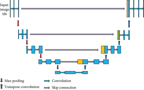
To the best of our knowledge, it is the first time that the “U-net” is used as a feature extractor in the area of equipment faulty prognostic. Normally, the U-net-based CNN network consists of two parts, the max-pooling period in the left and the upconvolution period in the right which jointly construct the “U” structure as shown in Figure 1. It usually consist of four kinds of operations, namely, convolution, max-pooling, transpose-convolution, and skip connection.

Details are in the caption following the image — **Figure 1**
Open in figure viewer PowerPoint

The conventional U-net structure.

2.1.1. Convolution Operation

The convolution layer consists of a series of feature maps which is obtained through the convolution operation between the convolution kernel and the input as shown in

(1)

denotes the α_th output feature map of the j_th layer;

denotes the β_th input feature map of the (j − 1)_th layer;

denotes the convolution kernel between the feature map

and the feature map

. The f(∗) denotes the activation function. In order to increase the nonlinearity of CNN, the rectifier linear units (Relu) is adopted in this paper due to its excellent performance. The ReLu function can be expressed as shown in

(2)

2.1.2. Max-Pooling Operation

In order to release the model parameter size as well as the overfitting problem, the pooling operation is executed along with the convolution operation. Since the convolution kernels for the same feature map share the same weight and bias, a max-pooling layer is added to each convolution layer, producing lower resolution feature maps through subsampling operations. The max-pooling function can be defined as illustrated in

(3)

where the

and

denote the S₁∗S₂ pixel in the a_th feature map before and after max-pooling operation. The parameter λ denotes the stride size of the pooling window whose value should be larger than 1. The max-pooling operation decreases the size of the feature maps and subsamples the highest resolution proportion of the input feature image which greatly reduce the parameter number of the CNN model.

2.1.3. Transpose Convolution

In order to obtain the feature image which has the same size as the input image, the transpose convolution operation is applied along with the max-pooling process. During the transpose convolution process, the domain interpolation is the most commonly used technology as shown in

(4)

where the

denotes the i∗i pixel value in the a_th feature map before the transpose convolution operation and

denotes the I∗I pixel value in the a_th feature image after the transpose convolution operation; the parameter S denotes the stride step of the transpose convolution, and the parameter p denotes the zero padding. The kernel size of the transpose convolution kernel is k∗k.

2.1.4. Skip Connection

The U-net is a typical encoding-decoding structure. The encoding process is realized by the max-pooling operation while the decoding process is realized by the transpose convolution operation. In order to compensate the information loss during the max-pooling process, the U-net utilizes the concatenation layer to realize the feature fusion of the two symmetrical feature images located in the max-pooling and transpose processes, respectively, which is called skip connection. The “skip connection” enhances the hierarchical feature learning ability of the U-net without resolution loss.

2.2. Attention Learning and CBAM

The attention learning is first inspired by the cognitive neuroscience. When dealing with a certain task, people will pay more attention to the important issue while paying less attention to the unimportant ones. Based on this notion, the attention mechanism is first proposed by Treisman and Gelade in 1980s [35]. The attention mechanism is aimed at assigning different weights to different proportions of the input based on the contribution of the different input proportions to the output. It has already been successfully applied into the area of natural language processing, machine translation, pattern recognition, and large equipment maintenance due to its powerful ability of extracting discriminative features [36].

Chen et al. [37] proposed an attention-based deep learning framework for machine’s RUL prediction. In his paper, the proposed approach first exploits the LSTM network to learn representative sequential features from raw sensory data, then the attention learning network is utilized to learn the importance of the sequential features and assign larger weights to more important ones. Chen et al. [38] applied a spatial-temporal convolution neural network with convolution block attention module for microexpression recognition. First image sequences were input to a medium-sized convolution neural network (CNN) to extract visual features. Afterwards, it learned to allocate the feature weights in an adaptive manner with the help of a convolutional block attention module. Since microexpressions only occur in parts of the human face, the attention mechanism helps to focus on specific facial regions, learning and acquiring the important features. Xiong et al. [39] proposed an attention augmented multiscale network (AAMN) for single-image superresolution (SISR), employing an attention driven strategy to guide feature selection and aggregation among multiple branches. Leng et al. [40] proposed a context-aware attention network combining the context learning module and the attention transfer module. The context learning module is first utilized to capture the global contexts. Then, the attention transfer module is proposed to generate attention maps that contain different attention regions, benefiting for extracting discriminative features.

Currently, there are two most commonly used attention learning mechanism, namely, SENET (sequential and excitation network) and CBAM (convolutional block attention model) [37]. The SENET applies the attention module to channel dimension while the CBAM applies the attention module not only on the channel dimension but also the spatial dimension of the image.

The idea of the CBAM attention mechanism was first proposed by Woo et al. [36]. The CBAM consists of channel attention process and spatial attention process as shown in Figure 2. The overview of the channel-spatial process of the CBAM is illustrated in

(5)

where M represents the input image of the CBAM module with the channel number of C, the height of H, and the width of W. The mark ⊗represents the element-wise multiplication, M^′ represents the feature image multiplying the channel attention map, and M^″ represents the result of the spatial attention map multiplying M^′ which is regarded as the output of the CBAM module.

2.2.1. Channel Attention Process

Usually, the input image can be transferred to a feature matrix through the convolutional layer. The channel number of the obtained feature matrix is the same as the kernel number of the convolutional layer with the common value of 256 or 512. Since some channels are not so useful to the information transference, it is necessary to apply channel attention on these channels. The attention weighting process is illustrated in

(6)

where the

and

denote the average pooling operation and the max pooling operation applied on the channel dimension of the feature matrix. W₀ ∈ R^C/r∗C and W₁ ∈ R^C∗C/r denote the activation operation of the shared multilayer perceptron with activation function of rectified linear unit (Relu) with the size of R^C/r∗1∗1,where r denotes the compression ratio.The parameter σ denotes the sigmoid activation.

2.2.2. Spatial Attention Process

Similar as the channel attention process, the spatial attention is aimed at applying the importance weighting on spatial dimension of the feature matrix as shown in

(7)

where the average pooling and the max pooling are also applied for the information evaluation. The parameter f^R∗R denotes the convolutional layer with the kernel size of ∗R and the spatial attention weighting is finally normalized by the sigmoid activation.

2.3. Proposed Combination Model Based on U-Net and CBAM Mechanism

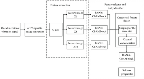
Although the hierarchical feature extraction network can provide the multilevel characteristics of the input image, the input image has been largely expanded to some extent. Therefore, it is necessary to use the attention learning network to capture the sensitive proportion of these input feature images and eliminate the abundant proportion. This paper proposes a hybrid model based on the U-net and the CBAM-based attention learning blocks, compromising the hierarchical feature extraction of the U-net, the attention learning of the CBAM blocks, and the effectiveness of the combination. The overall framework is illustrated in Figure 3.

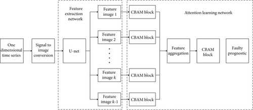
Firstly, the one-dimensional time series signal has been converted into the two dimensional gray-scale image, which is then decomposed by the U-net into several multilevel feature images hierarchically, representing the hierarchical characteristics of the input signal.

Secondly, multiple CBAM attention learning blocks are used to optimize the decomposed features, selecting the faulty sensitive features from the redundant ones. The complexity of the hierarchical feature images are greatly reduced, thus promoting the prediction efficiency.

Finally, the outputs of the CBAM attention learning blocks are aggregated, and the second CBAM block is applied on the categorical feature image. The categorical feature optimized by the CBAM attention learning is sent to the Softmax layer for final faulty prognostic as shown in

(8)

where C⁽ⁱ⁾ denotes the optimized categorical feature image used for faulty prognostic; i = 1, 2..n denotes the number of the training data; j = 1, 2..k denotes the dimension of the output layer which is equal to the faulty type number. θ denotes the parameters of the Softmax layer.

3. Proposed Faulty Prognostic Procedure

3.1. Data Preprocessing

Generally speaking, the condition monitoring data collected from the front-end industrial equipment includes one-dimensional time series data and two-dimensional image data. The 2D image data can be used directly for the faulty prognostic task by using the pattern recognition techniques. In this paper, we use the “N∗N” signal to image conversion technique proposed in literature [41] to convert the 1D time series vibration signal data into the 2D image data; the converted image is used as the input of the U-net convolution neural network. The specific schematic diagram of the N∗N “signal to image” conversion process is illustrated in Figure 4.

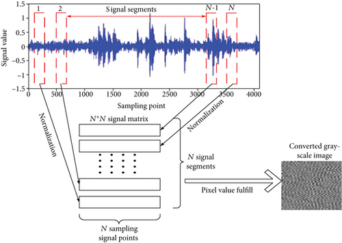
First, we randomly choose N signal segments from the raw signal containing N sampling points in each segment equally. Since the maximum value of the pixel length of the gray image is less than 255, the selected N² sampling points are normalized into the value ranging from 0~255 by using Equation (9) and the N∗N signal matrix is constructed. Finally, the normalized pixel value of the signal matrix is fulfilled for the construction of the gray-scale image.

(9)

In Equation (9), the round function transforms the sampling signal value to the gray scale pixel value by using the round function “round(∗)”. The Pixel(i, j) denotes the converted pixel value of the corresponding signal value(i, j) where the min (value) denotes the minimum value of sampling data point among the selected N² sampling data point while the max (value) denotes the maximum value among the N² data points. The above “signal to image” conversion method used in this paper is simple, and it has been proved to be effective in literature [41] due to its less requirement of the domain expertise and signal processing knowledge. The converted gray-scale image is a 2D representation of the raw signal which can effectively retain the details and characteristics of the raw signals.

3.2. Proposed Feature Extraction Network and Attention Learning Block

3.2.1. Proposed U-net-Based Feature Extraction Network

In this paper, a U-net-based convolution neural network is designed as the hierarchical feature extraction network. The whole feature extraction network consists of 10 layers, namely, X1~X10, among which the feature images of X1~X4 denote the max-pooling process of the U-net while the feature images of X5~X10 denote the upconvolution process of the U-net as shown in Figure 5.

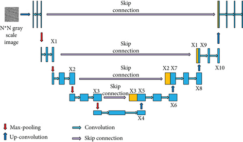
Since the feature layers of the transposed process of the U-net can better represent the hierarchical characteristics of the input data which contains less outside noise, the feature layers of X6, X8, and X10 from the low, middle, and high levels, respectively, are used as the extracted hierarchical features, representing the global and specific characteristics of different health conditions, thus contributing different knowledge to the feature extraction task.

3.2.2. Proposed ResNet-CBAM Attention Learning Block

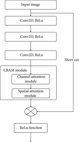
In this paper, the designed CBAM attention learning network is compiled with the three-layer ResNet CNN as shown in Figure 6. First, the ResNet-based CNN is used to extract the spatial and channel features of the input feature images. Then, the CBAM attention learning block is used for the attention weighting of the channel dimensions and the spatial dimensions of the input images in an adaptive way. The advantage of the proposed ResNet-CBAM attention learning block is that there will not be feature loss and gradient disappearance before the input images are processed by the CBAM module.

3.2.3. Proposed Prognostic Procedure

The proposed prognostic procedure is illustrated in Figure 7. First, the one-dimensional time series data is converted to the two-dimensional gray-scale image by using the “N∗N” image conversion approach. Second, the U-net-based hierarchical feature extraction network is applied and the multilevel feature images of X6, X8, and X10 are extracted as the multi-input of the attention learning network. Third, the three designed ResNet-CBAM-based attention learning blocks are applied on the three extracted multilevel feature images which are then fused through shaping into the same size and channel concatenation. Finally, the concatenated categorical feature image is optimized by the second ResNet-CBAM attention learning block, and the final faulty prognostic result can be calculated through Softmax prediction. The novel Pareto-optimal strategy based on spatial game theory which is proposed by Wong [42–43] is utilized as the parameter optimization strategy of the proposed hybrid faulty prognostic model. The general procedure of the proposed approach is illustrated in Algorithm 1.

Algorithm 1: The general procedure of the proposed methodology.

Algorithm: General procedure of the proposed approach
Input: Given the one-dimensional time series bearing vibration data samples of different faulty diameters under different working loads, the architecture and parameters of the proposed U-net and the designed CBAM attention learning model.
Output: The prediction result and the testing accuracy.
Step 1: Generate the training datasets and the testing datasets
1.1: Obtain the gray scale images of the one dimensional time series samples of the vibration signal by using the N∗N signal-to-image conversion method.
1.2: Categorized the gray scale images into the training datasets Xs and the testing datasets Xt.
Step 2: Construct the U-net hierarchical feature extractor for multilevel feature extraction
2.1: Construct the U-net hierarchical feature extractor as shown in Figure 5 and input the training datasets of Xs.
2.2: Train the U-net hierarchical feature extractor by using unsupervised training.
2.3: Extract the multilevel feature images of X6, X8, and X10 in the upconvolution process of the U-net.
Step 3: Construct the attention learning mechanism for the further feature optimization
3.1: Construct the ResNet-CBAM-based attention learning network as shown in Figure 7 and apply it for the further feature optimization of the feature images X6, X8, and X10, respectively.
3.2: Applying shaping and concatenation process for the construction of categorical feature.
3.3: Applying ResNet-CBAM feature extraction network for the second feature optimization of the categorical feature in procedure 3.2.
Step 4: Output the faulty prognostic result using flatten, dense, and Softmax prediction
4.1: Applying flatten, dense processing for the output in procedure 3.3.
4.2: Applying Softmax prediction using Equation (8) for calculating the final faulty prognostic result.
4.3: Optimizing the parameter of the proposed approach through minimizing the loss function in Equation (12) by using spatial game theory-based Pareto-optimal strategy.
4.4: Repeat the procedures from 2.1 to 4.3 and finish the training procedure.
Step 5: Evaluate the proposed methodology
Evaluate the performance of the proposed methodology on testing datasets Xt and output the testing accuracy of the proposed approach.

3.3. Performance Metrics

In order to evaluate the prediction accuracy as well as the prediction efficiency of the proposed approach, the “accuracy” metric, the “accuracy gain” metric, and the function of the “average accuracy gain” are used in this paper.

Equation (10) denotes the definition of the “accuracy” function which has been widely used in the accuracy evaluation of the classifying problem including the faulty classification task mentioned in this paper.

(10)

where m denotes the number of the training or testing samples per epoch;

denotes the prognostic value obtained by model, and y_i denotes the true label.

Equation (11) denotes the definition of the accuracy gain (AG) and the average accuracy gain (AAG) which has been frequently used to evaluate the speed-up properties of the prediction model [44].

(11)

where the

and

denote the achieved accuracy of model 1 and model 2, respectively, after the i_th epoch; AG_i denotes the accuracy gain of model 1 over model 2 after the i_th epoch;

denotes the average accuracy gain of model 1 over model 2 within the epoch range of N_epoch; the indicator AG_i evaluates the model speed-up properties from the microperspective while the indicator

evaluates the model speed-up properties from the macroperspective.

The loss function is defined as shown in Equation (12), where I(∗) denotes the indicator function and N denotes the number of the training samples.

(12)

4. Methodology Evaluation

In order to evaluate the effectiveness of the proposed approach, two case studies are adopted with two bearing datasets from the reliance electric motor and electromechanical drive system, respectively. The experimental environment of this paper is Intel Xeon 5238 [email protected] Hz x 2, 1 T SSD, 4xTesla T4 GPU, 256 G running memory.

4.1. Case Study 1: Bearing Faulty Prognostic for Reliance Electric Motor

4.1.1. Data Description and Experimental Set-Up

Performance of the proposed approach is evaluated on the bearing fault datasets provided by the CWRU (Case Western Reserved University) bearing data center [45]. The vibration signal data is collected from the drive-end of a 2-hp reliance electric motor as shown in Figure 8.

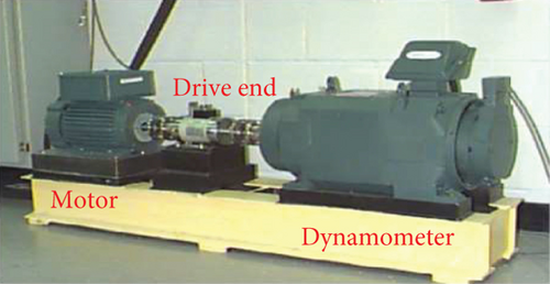
The accelerator sensors are installed on the inner race, ball, and the outer race, respectively. In this case study, only the data collected from the inner race are collected and analyzed. The vibration data is sampled at the frequency of 12 kHz under different rotating speed of 1730 rpm, 1750 rpm, 1772 rpm, and 1797 rpm. There are totally five statuses of the inner race including one normal status and four different faulty severity statuses of the diameters 0.007, 0.014, 0.021, and 0.028, respectively. Therefore, five operating statuses are included in the datasets.

In this experiment, two datasets including the training datasets and the testing datasets in each are generated, respectively. In dataset Ι, for each health condition, 100 samples with 4096 data points in each sample are randomly selected under each load condition in the training datasets. That is to say, there are 400 samples of a single health condition with the load condition of 0, 1, 2, and 3. Therefore, there are totally 2000 samples of five health conditions altogether. Meanwhile, 2000 samples are randomly selected in the same way for the testing datasets. In dataset II, the training and testing samples are selected under different loads where 1500 samples with five operating statuses are randomly selected under the load condition of 0, 1, and 2 as the training datasets, while the testing datasets consist of 500 samples of five operating status under the load condition of 3. More details of the two datasets, namely, dataset I and dataset II, are listed in Table 1.

Table 1. The details of the two bearing datasets.

Machine operating status type	Class label	Dataset I number of training (loads: 0-3)/testing (loads: 0-3) samples	Dataset II number of training (loads: 0-2)/testing (loads: 3) samples
Normal	0	400/400	300/100
Faulty diameter 0.007	1	400/400	300/100
Faulty diameter 0.014	2	400/400	300/100
Faulty diameter 0.021	3	400/400	300/100
Faulty diameter 0.028	4	400/400	300/100

4.1.2. Results and Discussion

The raw vibration signal is converted to the N∗N gray-scale image by using the N∗N conversion approach. Since each sample contains 4096 signal points, the scale size of the gray scale image is set to the size of 64∗64. The converted gray-scale image of five operating status under load 0 are shown in Figure 9. It can be found that there is naked-eye distinguishable differences among these converted gray-scale images, which is applicable for the input of the U-net.

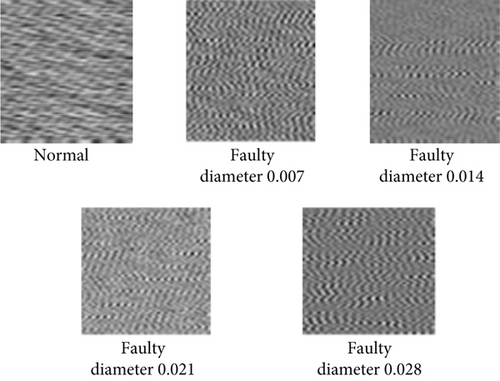
The converted (64∗64) gray-scale images are used as the input of the U-net-based hierarchical feature extraction network with the specific configuration as shown in Table 2, where the feature layers of X6 (512@8∗8), X8 (256@16∗16), and X10 (128@32∗32) are extracted, respectively.

Table 2. The detailed structure of the U-net model.

Layer name	Configuration	Kernel/pooling/transpose size
Input	64∗64
X1	128@32∗32	128@3∗3
X2	256@16∗16	256@3∗3
X3	512@8∗8	512@3∗3
X4	1024@4∗4	1024@3∗3
X5	512@8∗8	2∗2
X6	512@8∗8	512@3∗3
X7	256@16∗16	2∗2
X8	256@16∗16	256@3∗3
X9	128@32∗32	2∗2
X10	128@32∗32	128@3∗3

In order to demonstrate the generalization ability and the faulty sensitivity of the proposed U-net hierarchical feature extractor, the t-distributed stochastic neighbor embedding (t-SNE) technology, regarded as a novel technology which visualizes high-dimensional data by giving each data-point a location in a two- or three-dimensional map [46], is used here for the visualized evaluation of the U-net hierarchical feature extractor. As shown in Figures 10(a)–10(f), the two-dimensional visualizations of the feature images X6, X8, and X10 are illustrated under the test set of dataset I (loads 0~3) and the test set of dataset II (load 3), where different colors represent different health conditions.

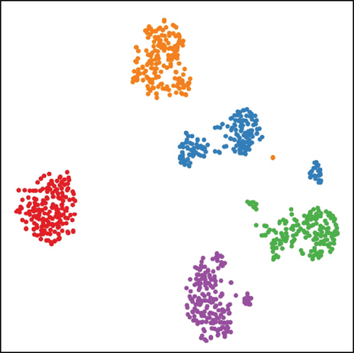
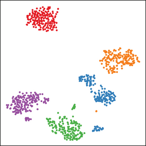
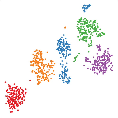
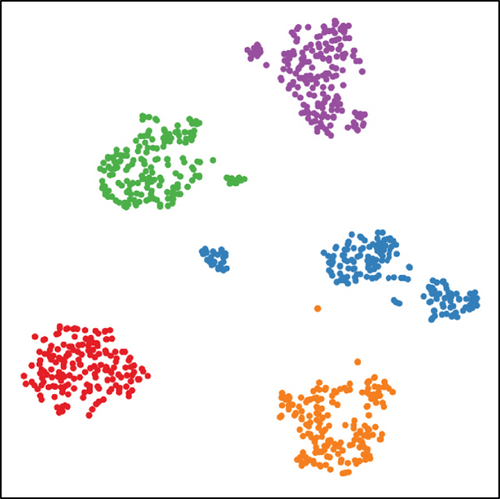
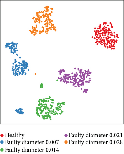
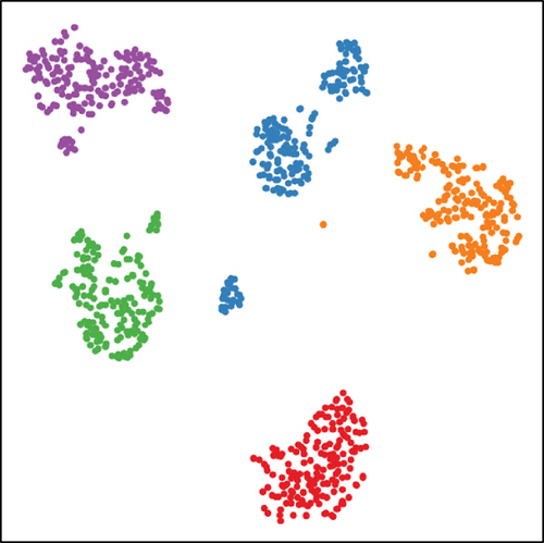
Firstly, it can be found that the vast majority of the samples belonging to the same conditions are well gathered while separated for different health conditions. Therefore it can be concluded that the extracted multilevel features of the U-net feature extractor can be very sensitive for the faulty information contained in the gray-scale image. By the comparison analysis in Figures 10(a)–10(f), it is worth mentioning that the majority of samples belonging to the same health condition can be well gathered in the test set of both datasets, and there is no obvious difference in terms of the classification result. Since the operation conditions of the training and testing datasets are the same in dataset I while different in dataset II, it can be further proved that the U-net-based CNN has powerful generalized feature extraction ability which can be less influenced by the load condition variation.

In addition, the two-dimensional visualization view of the extracted multilevel features of X6, X8, and X10 are different from each other, indicating that the different feature level can contribute different knowledge to the faulty prognostic tasks. Therefore, it can be concluded the U-net-based CNN has powerful hierarchical feature learning ability which represent the information of the different health conditions from multiple aspects.

The visualization view of the representative feature images of X6, X8, and X10 is illustrated in Figure 11. It can be found that the three extracted multilevel feature images can be well distinguished from each other under the five different health statuses of the testing set of dataset I, indicating the proposed U-net hierarchical feature extractor being sensitive to the faulty information contained in the gray-scale feature image.

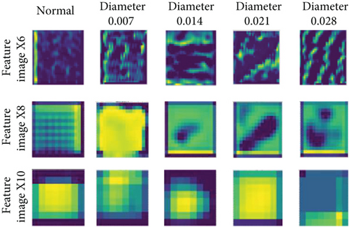
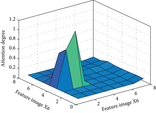
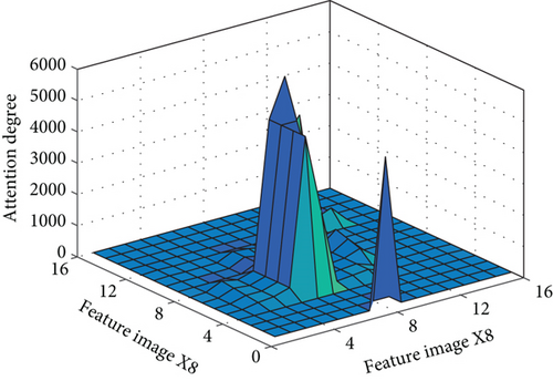
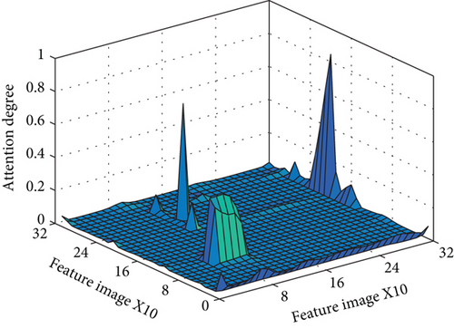
The extracted hierarchical features in layer X6, X8, and X10 are sent to the designed ResNet-CBAM attention learning block separately, and the designed ResNet-CBAM attention learning network is applied two times not only on the multilevel feature images but also on the (8∗8) concatenated categorical feature images. The visualization of the attention learning result of the health condition of faulty diameter 0.007 under load 0 is illustrated as shown in Figures 12(a)–12(d); it should be noted that there is obvious discriminative concentration on these extracted multilevel feature images and the concatenated categorical feature image, thus, assigning larger weights to the important features and promoting the prognostic efficiency as well as the prognostic accuracy. Therefore, it can be concluded that it is necessary to apply the CBAM attention learning block not only on the extracted multilevel features of X6, X8, and X10 but also on the concatenated categorical feature used for faulty prognostic.

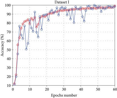
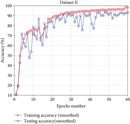
The optimized categorical feature image is sent to the Softmax layer for final faulty prognostic. The maximum epoch number is set to 60, and the average accuracy of the last 10 epochs from the 50^th to the 60^th epoch is defined as the final convergence accuracy (FCA) in this paper; the optimizer is Adam with the learning rate of 0.005. The prediction accuracy of the training and validation curves of two datasets are illustrated in Figure 13. It can be clearly seen that both the training and testing accuracy can reach almost 100% after the 60^th epoch in dataset I. In dataset II, the final convergence accuracy of the training result can also reach nearly 100%, and the testing accuracy can reach nearly 93%,which can be also comparatively high. Since the training and the testing datasets are collected under the same load in dataset Ι while different in dataset II, it can be proved that the proposed faulty prediction approach can achieve perfect prognostic accuracy as well as generalization ability.

4.1.3. Ablation Experiment

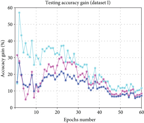
To evaluate the speed-up property promotion of introducing the attention mechanism to the proposed faulty prognostic framework, an ablation experiment of the different combinations of the U-net and the attention learning mechanism is evaluated on the two datasets of the case study. Specifically, we implement the proposed approach: the U-net+Softmax (US), the U-net+categorical attention+Softmax (UCAS) and the U-net+multi-scale attention+Softmax (UMAS). The “U-net+Softmax”, which has no attention learning process, is used as the benchmark model, and the performance metrics of accuracy gain and the average accuracy gain is adopted for the evaluation of the model speed-up properties promoted by the attention learning network. As shown in Figure 14, the proposed model which has two times attention learning process significantly outperform the US model especially in the first 30 epochs in terms of the testing accuracy gain of both datasets, which is very important for the real-time requirement of the practical industry during the infant stage. Moreover, the ablation models of the UCAS and UMAS, which have only one attention learning process on the categorical feature and the multiscale features, respectively, also have certain accuracy gain promotion compared with the US model, indicating the effectiveness of the introduction of the attention learning mechanism in promoting prediction efficiency.

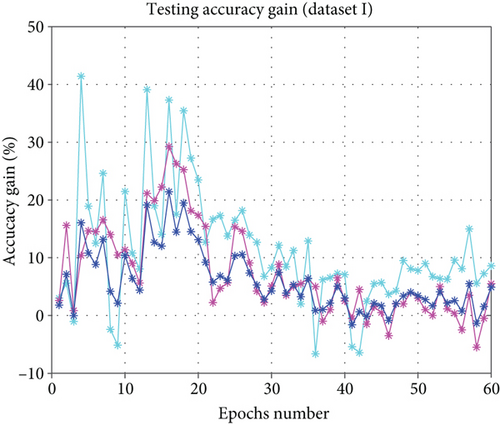
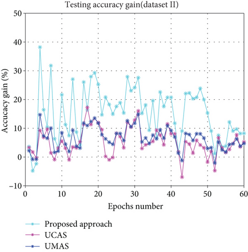
The ablation experiment is executed 10 times, and the mean values of the average final convergence accuracy (FCA) and the average accuracy gain (AAG) are illustrated in Table 3, where the proposed approach outperforms the other three ablation models in both metrics.

Table 3. Mean value of the final convergence accuracy and the average accuracy gain of the testing result on two datasets.

Model	Dataset I testing		Dataset II testing
Model	FCA	AAG	FCA	AAG
Proposed approach	98.59%	11.2%	93.24%	15.36%
U-net+categorical attention+Softmax	95.50%	7.45%	90.25%	5.23%
U-net+multiscale attention+Softmax	94.89%	5.97%	89.68%	6.42%
U-net+Softmax	90.00%	0%	85.50%	0%

4.1.4. Comparison Experiment

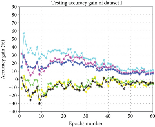
To further evaluate the speed-up properties of the attention learning network and the generalization ability of the U-net CNN-based hierarchical feature extractor, the comparison analysis introduces the proposed approach; the three ablation models as well as some hybrid prediction models based on the hierarchical feature extractor of the classical LeNet-5 CNN, namely, LeNet-5+Random forest (L-RF), LeNet-5+SVM(L-SVM), and LeNet-5+Softmax(LS) for comparison. Similar as the ablation experiment, the model of the U-net+Softmax is set as the benchmark model, and the accuracy gain curves of the multiple hybrid prediction approaches are illustrated in Figure 15, where the approaches with the attention learning mechanism has superior accuracy gain over the US model while the models without attention learning mechanism has inferior accuracy gain over US model, indicating the prognostic efficiency promotion of the attention learning.

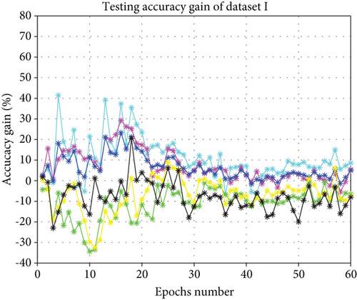
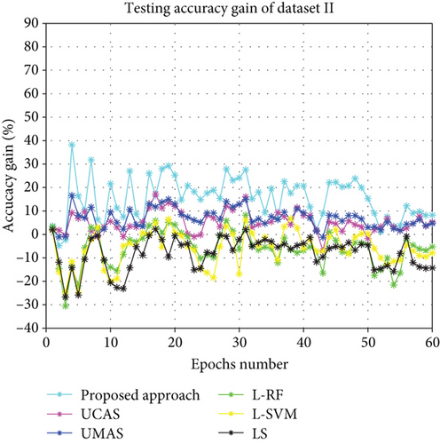
The comparison experiments are conducted 10 times on both datasets just the same as the ablation experiment. It can be clearly seen from Table 4 that the proposed approach achieves the highest final convergence accuracy and the most superior average accuracy gain on the testing result of both datasets. Moreover, it should be noted that the models with the U-net feature extractor network significantly outperform other traditional LeNet-5 CNN-based model especially on the final convergence accuracy of dataset II when compared with the performance on dataset Ι. Therefore, it can be concluded that the models with the designed U-net-based hierarchical feature extraction network has much better generalization ability compared with classical LeNet-5 CNN feature extractor network.

Table 4. The comparison result with other traditional approaches.

Model	Dataset I testing		Dataset II testing
Model	FCA	AAG	FCA	AAG
Proposed approach	98.58%	11.2%	93.24%	15.36%
U-net CNN+categorical attention+Softmax (UCAS)	95.5%	7.45%	90.25%	5.23%
U-net+multiscale attention+Softmax (UMAS)	94.89%	5.97%	89.68%	6.42%
U-net+Softmax (US)	90.00%	0%	85.50%	0%
LeNet-5 CNN+random forest (L-RF)	83.53%	-11.03%	79.71%	-6.01%
LeNet-5 CNN+SVM (L-SVM)	82.66%	-6.96%	77.1%	-5.83%
LeNet-5 CNN+Softmax (LS)	82%	-7.51%	70.73%	-8.09%

4.2. Case Study 2: Bearing Faulty Prognostic for Electromechanical Drive System

4.2.1. Data Description and Experimental Set-Up

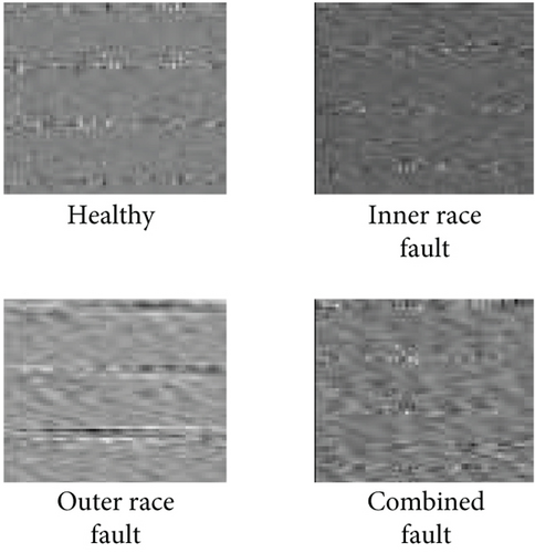
Performance of the proposed approach is evaluated on the bearing fault datasets provided by the Paderborn University [47]. The testing rig is illustrated in Figure 16 which consists of an electric motor (1), a torque-measurement shaft (2), a rolling bearing test (3), a flywheel (4), and a load motor (5). The experiment uses the motor current signal of the electromechanical drive system for bearing diagnostics which is collected under four operating conditions with different operating parameters settings as shown in Table 5. There are totally four different statuses of the electromechanical drive system, namely, inner-ring damage, outer-ring damage, combined damage, and the healthy status. All the samples with 4096 data sampling points are randomly selected from the conditional monitoring data. Different from the component faulty intensity classification of case study I, the faulty classification task in case study II involves multiple components. The arrangement of the training and testing datasets are illustrated in Table 6.

Table 5. The operating parameters of the four operating conditions.

Loads	Rotational speed [rpm]	Load torque [N∗m]	Radial force [N]	Name of setting
0	1500	0.7	1000	N15_M07_F10
1	900	0.7	1000	N09_M07_F10
2	1500	0.1	1000	N15_M01_F10
3	1500	0.7	400	N15_M07_F04

Table 6. The description of the evaluated datasets.

Machine operating status type	Class label	Dataset I number of training (loads: 0-3)/testing (loads: 0-3) samples	Dataset II number of training (loads: 0-2)/testing (loads: 3) samples
Healthy	1	400/400	300/100
Outer-ring damage	2	400/400	300/100
Inner-ring damage	3	400/400	300/100
Combined damage	4	400/400	300/100

4.2.2. Results and Discussion

In this experiment, the 4096 continuous signal points are converted to the 64∗64 gray-scale image the same as case study one. The conversion result of the four operating statuses under load 0 are illustrated in Figure 17. It can be concluded that these images corresponding to different health conditions can also differ from each other, and it should be easy to classify them which further proves the effectiveness of the “N∗N” signal to image conversion method.

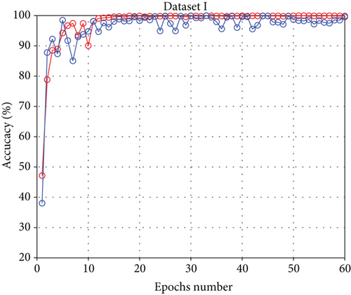
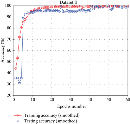
The same as the case study one, the converted gray-scale images are used as the input of the U-net feature extractor and the multilayer features extracted from the U-net are used as the input of the attention learning network for faulty classification within the maximum epoch range of 60. The prediction result is illustrated in Figure 18. It can be seen that the training and the testing accuracy of the 60^th epoch can reach nearly 100% on both datasets which can be comparatively higher than case study one. The reason should be that the classification task is only within the same component of inner-race faulty in case study one while including different components in case study two, which has more distinguishable faulty symptom.

4.2.3. Ablation Analysis

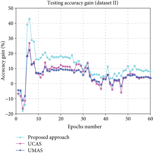
The AG curves illustrated in Figure 19 show the effectiveness of the attention learning network where the proposed approach, the UCAS, and the UMAS have obvious accuracy advantage over the U-net+Softmax within the same epoch range during the infant stage, indicating the effectiveness of the attention learning mechanism being also valid in case study two. The mean value of the average accuracy gain and the final convergence accuracy are illustrated in Table 7, where the proposed approach outperforms the other three ablation models in terms of both metrics in case study two.

Table 7. The comparison result of the ablation experiment.

Model	Dataset Ι testing		Dataset II testing
Model	FCA	AAG	FCA	AAG
Proposed approach	99.56%	24.17%	98.87%	11.49%
U-net+categorical attention+Softmax	96.31%	16.52%	94.47%	5.78%
U-net+multiscale attention+Softmax	95.01%	13.57%	94.68%	5.52%
U-net+Softmax	87.85%	0%	90.9%	0%

4.2.4. Comparison with Other Approaches

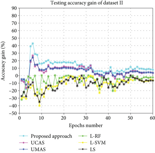
Figure 20 and Table 8 show the accuracy gain curve; the mean final convergence accuracy and mean average accuracy gain of the proposed approach, the three ablation models and the traditional hybrid prediction models based on LeNet-5 hierarchical feature extractor network, where the model with the U-net feature extractor has better generalization ability; and the model with the attention learning mechanism has better speed-up properties especially during the infant stage, showing the great potential of the U-net, the attention learning network, and the proposed combination.

Table 8. The comparison result with other traditional approaches.

Model	Dataset I		Dataset II
Model	FCA	AAG	FCA	AAG
Proposed approach	99.56%	24.17%	98.87%	11.49%
U-net CNN+categorical attention+Softmax (UCAS)	96.31%	16.52%	94.47%	5.78%
U-net+multiscale attention+Softmax (UMAS)	95.01%	13.57%	94.68%	5.52%
U-net+Softmax (US)	87.85%	0%	90.9%	0%
LeNet-5 CNN+random forest (L-RF)	82.14%	-5.1%	85.51%	-6%
LeNet-5 CNN+SVM (L-SVM)	83.5%	-7.95%	84.64%	-10.96%
LeNet-5 CNN+Softmax (LS)	83.3%	-8.46%	84.35%	-11.31%

5. Conclusion and Future Work

5.1. Main Contribution of the Proposed Paper

In this paper, a novel bearing faulty prediction approach based on the U-net-based hierarchical feature extractor network and the ResNet-CBAM-based attention learning network is proposed. The main contributions of this paper can be summarized as follows:

(1)
Introducing the N∗N “signal to image” conversion approach, the N∗N data to image approach can be simple but effective which can relax the dependencies on the domain expertise knowledge of signal processing
(2)
Proposing a U-net CNN-based multilevel feature extractor network which has powerful generalized and hierarchical feature extraction ability. The extracted multilevel features can distinguish the different health conditions under the complex operational conditions and represent the different health conditions from multiple aspects, contributing different knowledge to the prognostic tasks
(3)
Applying the designed ResNet-CBAM-based attention learning network for the feature selection of the extracted features. The ResNet-CBAM block is applied two times not only on the multilevel feature images but also on the categorical feature image. There is obvious discriminative concentration on the extracted features, and the proposed hybrid model can achieve certain prediction accuracy within the limited epoch range, enhancing the model speed-up properties
(4)
Proposing the combination framework of the U-net and the ResNet-CBAM attention learning network. The U-net is used as the feature extractor, and the attention learning network is used as the feature selector and faulty classifier. Both the generalization ability and the speed-up properties of the model have been improved

The proposed approach is validated on two case studies, namely, offered by the CWRU (Case Western Reserved University) and the Paderborn University. Both case studies prove the effectiveness of the generalization ability of the U-net and the speed-up properties of the attention learning network. Moreover, the proposed approach is validated on the ablation experiment and the comparison experiment which further proves the effectiveness of introducing the proposed combination of the U-net and the attention learning network.

5.2. Future Work of the Proposed Paper

Although the proposed approach has made some achievements, there are still two items needed to be considered. Firstly, the complexity of the U-net-based hierarchical feature learning network as well as the attention learning network should be taken into account. In the future, the parameter scale of the proposed approach should be shortened which can be applicable for the model deployment of the edge-computing devices. Moreover, the proposed bearing faulty classification approach should be expected to be widely used in the faulty classification of other similar prognostic scene such as the gearbox, the milling equipment, and the gas pump system.

Conflicts of Interest

The authors declare that there are no conflicts of interest regarding the publication of this article.

Acknowledgments

This research has been financially supported by the “Science and Technology Innovation 2030-The Significant Project of a New Generation of Artificial Intelligence (2018AAA0101801)”.

Open Research

Data Availability

The dataset used to support the findings of this paper have been deposited in the CWRU (Case Western Reserved datasets) with the link of “https://csegroups.case.edu/bearingdatacenter/pages/12k-drive-end-bearing-fault-data” and the Paderborn University with the link of “http://groups.uni-paderborn.de/kat/BearingDataCenter/.”

References

1 Hong L. and Dhupia J. S., A time domain approach to diagnose gearbox fault based on measured vibration signals, Journal of Sound and Vibration. (2014) 333, no. 7, 2164–2180, https://doi.org/10.1016/j.jsv.2013.11.033, 2-s2.0-84892609656.
10.1016/j.jsv.2013.11.033
Web of Science® Google Scholar
2 Borghesani P., Pennacchi P., and Chatterton S., The relationship between kurtosis- and envelope-based indexes for the diagnostic of rolling element bearings, Mechanical Systems and Signal Processing. (2014) 43, no. 1-2, 25–43, https://doi.org/10.1016/j.ymssp.2013.10.007, 2-s2.0-84889079481.
10.1016/j.ymssp.2013.10.007
Web of Science® Google Scholar
3 Garcia M. C., Sanz-Bobi M. A., and del Pico J., SIMAP: intelligent system for predictive maintenance: application to the health condition monitoring of a windturbine gearbox, Computers in Industry. (2006) 57, no. 6, 552–568, https://doi.org/10.1016/j.compind.2006.02.011, 2-s2.0-33746237617.
10.1016/j.compind.2006.02.011
Web of Science® Google Scholar
4 Coronado D. and Fisher K., Condition Monitoring of Wind turbines: State of the Art, User Experience and Recommendations, 2015, VGB Research Foundation,VGB-Nr.383; Fraunhofer-IWES Bremer haven, Germany.
Google Scholar
5 Asgarpour M. and Sørensen J., Bayesian based diagnostic model for condition based maintenance of offshore wind farms, Energies. (2018) 11, no. 2, https://doi.org/10.3390/en11020300, 2-s2.0-85054160124.
10.3390/en11020300
Web of Science® Google Scholar
6 Xu G., Liu M., Jiang Z., Shen W., and Huang C., Online fault diagnosis method based on transfer convolutional neural networks, IEEE Transactions on Instrumentation and Measurement. (2019) 69, 1–12.
Web of Science® Google Scholar
7 Xu X., Zhang C., Derazkola H. A., Demiral M., Zain A. M., and Khan A., UFSW tool pin profile effects on properties of aluminium-steel joint, Vacuum. (2021) 192, no. 8, article 110460, https://doi.org/10.1016/j.vacuum.2021.110460.
10.1016/j.vacuum.2021.110460
Web of Science® Google Scholar
8 Zhang X. X. C., Derazkola H. A., Demiral M., Zain A. M., and Khan A., Dispersion of waves characteristics of laminated composite nanoplate, Steel and Composite Structures. (2021) 40, no. 3, 355–367.
Web of Science® Google Scholar
9 Liu Z., Jia Z., Vong C. M., Bu S., Han J., and Tang X., Capturing high-discriminative fault features for electronics-rich analog system via deep learning, IEEE Transactions on Industrial Informatics. (2017) 13, no. 3, 1213–1226, https://doi.org/10.1109/TII.2017.2690940, 2-s2.0-85020682598.
10.1109/TII.2017.2690940
Web of Science® Google Scholar
10 Li H., Chen J., Lu H., and Chi Z., CNN for saliency detection with low-level feature integration, Neuro Computing. (2017) 226, 212–220, https://doi.org/10.1016/j.neucom.2016.11.056, 2-s2.0-85008256639.
10.1016/j.neucom.2016.11.056
Google Scholar
11 Tang Z., Zhao G., and Ouyang T., Two-phase deep learning model for short-term wind direction forecasting, Renewable Energy. (2021) 173, 1005–1016, https://doi.org/10.1016/j.renene.2021.04.041.
10.1016/j.renene.2021.04.041
Web of Science® Google Scholar
12 Shao H., Jiang H., Zhang X., and Niu M., Rolling bearing fault diagnosis using an optimization deep belief network, Measurement Science and Technology. (2015) 26, no. 11, article 11500, https://doi.org/10.1088/0957-0233/26/11/115002, 2-s2.0-84946064662.
10.1088/0957-0233/26/11/115002
Web of Science® Google Scholar
13 He M. and He D., Deep learning based approach for bearing fault diagnosis, IEEE Transactions on Industry Applications. (2017) 53, no. 3, 3057–3065, https://doi.org/10.1109/TIA.2017.2661250, 2-s2.0-85028852181.
10.1109/TIA.2017.2661250
Web of Science® Google Scholar
14 Qi Y., Shen C., Wang D., Shi J., Jiang X., and Zhu Z., Stacked sparse autoencoder-based deep network for fault diagnosis of rotating machinery, IEEE Access. (2017) 5, 15066–15079, https://doi.org/10.1109/ACCESS.2017.2728010, 2-s2.0-85028453210.
10.1109/ACCESS.2017.2728010
Web of Science® Google Scholar
15 Haidong S., Hongkai J., Xingqiu L., and Shuaipeng W., Intelligent fault diagnosis of rolling bearing using deep wavelet auto-encoder with extreme learning machine, Knowledge-Based Systems. (2018) 140, 1–14, https://doi.org/10.1016/j.knosys.2017.10.024, 2-s2.0-85035078800.
10.1016/j.knosys.2017.10.024
Web of Science® Google Scholar
16 Xia M., Li T., Xu L., Liu L., and de Silva C. W., Fault diagnosis for rotating machinery using multiple sensors and convolutional neural networks, IEEE/ASME Transactions on Mechatronics. (2018) 23, no. 1, 101–110, https://doi.org/10.1109/TMECH.2017.2728371, 2-s2.0-85028941380.
10.1109/TMECH.2017.2728371
Web of Science® Google Scholar
17 Lee K. B., Cheon S., and Kim C. O., A convolutional neural network for fault classification and diagnosis in semiconductor manufacturing processes, IEEE Transactions on Semiconductor Manufacturing. (2017) 30, no. 2, 135–142, https://doi.org/10.1109/TSM.2017.2676245, 2-s2.0-85018771617.
10.1109/TSM.2017.2676245
Web of Science® Google Scholar
18 Wen L., Gao L., and Li X., A new deep transfer learning based on sparse auto-encoder for fault diagnosis, IEEE Transactions on Systems, Man, and Cybernetics: Systems. (2019) 49, no. 1, 136–144.
10.1109/TSMC.2017.2754287
Web of Science® Google Scholar
19 Min X., Teng L., Lin X., Liu L., and de Silva C. W., Fault diagnosis for rotating machinery using multiple sensors and convolutional neural networks, IEEE/ASME Transactions on Mechatronics. (2017) 23, no. 1, 101–110.
Web of Science® Google Scholar
20 Ding X. and He Q., Energy-fluctuated multiscale feature learning with deep ConvNet for intelligent spindle bearing fault diagnosis, IEEE Transactions on Instrumentation and Measurement. (2017) 66, no. 8, 1926–1935, https://doi.org/10.1109/TIM.2017.2674738, 2-s2.0-85015852225.
10.1109/TIM.2017.2674738
Web of Science® Google Scholar
21 Sun Y., Wang X., and Tang X., Deep learning face representation from predicting 10, 000 classes, IEEE Conference on Computer Vision & Pattern Recognition, 2014, Columbus, OH, USA, 1891–1898.
Google Scholar
22 Lee J. and Nam J., Multi-level and multi-scale feature aggregation using pre-trained convolutional neural networks for music auto-tagging, IEEE Signal Processing Letters. (2017) 24, no. 8, 1208–1212, https://doi.org/10.1109/LSP.2017.2713830, 2-s2.0-85028368778.
10.1109/LSP.2017.2713830
Web of Science® Google Scholar
23 Xu G., Liu M., Jiang Z., Söffker D., and Shen W., Bearing fault diagnosis method based on deep convolutional neural network and random forest ensemble learning, Sensors. (2019) 19, no. 5, https://doi.org/10.3390/s19051088, 2-s2.0-85062430554, 30832449.
10.3390/s19051088
PubMed Web of Science® Google Scholar
24 LeCun Y., LeNet-5, convolutional neural networks, 2015, http://yann.lecun.com/exdb/lenet.2015.
Google Scholar
25 Krizhevsky A., Sutskever I., and Hinton G. E., Imagenet classification with deep convolutional neural networks, Advances in Neural Information Processing Systems. (2012) 25, 1097–1110.
Google Scholar
26 Simonyan K. and Zisserman A., Very deep convolutional networks for large-scale image recognition, 2014, https://arxiv.org/abs/1409.1556.
Google Scholar
27 Szegedy C., Wei L., Jia Y., Sermanet P., Reed S., Anguelov D., Erhan D., Vanhoucke V., and Rabinovich A., Going deeper with convolutions, Proceedings of the IEEE conference on computer vision and pattern recognition, 2014, Boston, MA, USA, 1–9.
Google Scholar
28 Ronneberger O., Fischer P., and Brox T., U-net: convolutional networks for biomedical image segmentation, International Conference on Medica image computing and computer-assisted intervention, 2015, Munich, Germany, 234–241.
Google Scholar
29 Zhao F., Wu Z., Wang L., Lin W., Gilmore J. H., Xia S., Shen D., and Li G., Spherical deformable U-net: application to cortical surface parcellation and development prediction, IEEE Transactions on Medical Imaging. (2021) 40, no. 4, 1217–1228, https://doi.org/10.1109/TMI.2021.3050072.
10.1109/TMI.2021.3050072
PubMed Web of Science® Google Scholar
30 Gao H., Qiu T., Yuanting C., Zhou M., and Zhang X., Blood vessel segmentation of fundus images based on improved U network, 2019 Chinese Automation Congress (CAC), 2019, Hangzhou, China, 4017–4021, https://doi.org/10.1109/CAC48633.2019.8996153.
10.1109/CAC48633.2019.8996153
Google Scholar
31 Lei X., Chen Y., Chang W., Zhan Y., Lin W., Wang Q., and Shen D., Ultra-Fast T2-Weighted MR Reconstruction Using Complementary T1-Weighted Information, 2018, Springer, Cham, Switzerland.
Google Scholar
32 Nazem F., Ghasemi F., Fassihi A., and Dehnavi A. M., 3D U-Net: a voxel-based method in binding site prediction of protein structure, Journal of Bioinformatics and Computational Biology. (2021) 19, no. 2, https://doi.org/10.1142/S0219720021500062.
10.1142/S0219720021500062
PubMed Web of Science® Google Scholar
33 Dogan R. O., Dogan H., Bayrak C., and Kayikcioglu T., A two-phase approach using mask R-CNN and 3D U-Net for high-accuracy automatic segmentation of pancreas in CT imaging, Computer Methods and Programs in Biomedicine. (2021) 207, article 106141, https://doi.org/10.1016/j.cmpb.2021.106141.
10.1016/j.cmpb.2021.106141
Web of Science® Google Scholar
34 Chae J., Hong K. Y., and Kim J., A pressure ulcer care system for remote medical assistance: residual U-Net with an attention model based for wound area segmentation, 2021, https://arxiv.org/abs/2101.09433.
Google Scholar
35 Treisman A. M. and Gelade G., A feature-integration theory of attention, Cognitive Psychology. (1980) 12, no. 1, 97–136, https://doi.org/10.1016/0010-0285(80)90005-5, 2-s2.0-0018878142.
10.1016/0010-0285(80)90005-5
CAS PubMed Web of Science® Google Scholar
36 Woo S., Park J., Lee J., and Kweon I. S., Cbam: convolutional block attention module, Proceedings of the 15th European Conference on Computer Vision, 2018, Munich,Germany, 3–19.
Google Scholar
37 Chen Z., Wu M., Zhao R., Guretno F., Yan R., and Li X., Machine remaining useful life prediction via an attention based deep learning approach, IEEE Transactions on Industrial Electronics. (2021) 68, https://doi.org/10.1109/TIE.2020.2972443.
10.1109/TIE.2020.2972443
Web of Science® Google Scholar
38 Chen B., Zhang Z., Liu N., Tan Y., Liu X., and Chen T., Spatiotemporal convolutional neural network with convolutional block attention module for micro-expression recognition, Information. (2020) 11, no. 8, https://doi.org/10.3390/info11080380.
10.3390/info11080380
Google Scholar
39 Xiong C., Shi X., Gao Z., and Wang G., Attention augmented multi-scale network for single image super-resolution, Applied Intelligence. (2021) 51, no. 2, 935–951, https://doi.org/10.1007/s10489-020-01869-z.
10.1007/s10489-020-01869-z
Web of Science® Google Scholar
40 Leng J., Liu Y., and Chen S., Context-aware attention network for image recognition, Neural Computing and Applications. (2019) 31, no. 12, 9295–9305, https://doi.org/10.1007/s00521-019-04281-y, 2-s2.0-85068050458.
10.1007/s00521-019-04281-y
Web of Science® Google Scholar
41 Wen L., Li X., Gao L., and Zhang Y., A new convolutional neural network-based data-driven fault diagnosis method, IEEE Transactions on Industrial Electronics. (2018) 65.
10.1109/TIE.2017.2774777
PubMed Web of Science® Google Scholar
42 Wong K. K., A geometrical perspective for the bargaining problem, PLoS One. (2010) 5, no. 4, article e10331, https://doi.org/10.1371/journal.pone.0010331, 2-s2.0-77956408195.
10.1371/journal.pone.0010331
Web of Science® Google Scholar
43 Wong K., Bridging game theory and the knapsack problem: a theoretical formulation, Journal of Engineering Mathematics. (2015) 91, no. 1, 177–192, https://doi.org/10.1007/s10665-014-9742-1, 2-s2.0-84925535946.
10.1007/s10665-014-9742-1
Web of Science® Google Scholar
44 Dong X., Wu H. H., Yan Y., and Qian L., Hierarchical transfer convolutional neural networks for image classification, 2019 IEEE International Conference on Big Data (Big Data), 2019, Los Angeles, CA, USA, 2817–2825, https://doi.org/10.1109/BigData47090.2019.9005707.
10.1109/BigData47090.2019.9005707
Google Scholar
45 Loparo K., Case Western Reserve University bearing data centre website, 2012, http://csegroups.case.edu/bearingdatacenter/pages/download-data-file.
Google Scholar
46 Shi S., Visualizing data using GTSNE, 2021, https://arxiv.org/abs/2108.01301.
Google Scholar
47 Lessmeier C., Kimotho J. K., Zimmer D., and Sextro W., Condition monitoring of bearing damage in electromechanical drive systems by using motor current signals of electric motors: a benchmark data set for data-driven classification, European Conference of the Prognostics and Health Management Society, 2016, Bilbao, Spain, 83–100.
Google Scholar

Citing Literature

All articles