Volume 2021, Issue 1 5815280

Research Article

Open Access

Short-Term Traffic Prediction considering Spatial-Temporal Characteristics of Freeway Flow

Jiaqi Wang

orcid.org/0000-0002-0891-1867

Department of Transportation Engineering, South China University of Technology, 381 Wushan Road, Guangzhou 510641, China scut.edu.cn

Search for more papers by this author

Yingying Ma,

Corresponding Author

Yingying Ma

[email protected]

orcid.org/0000-0002-3704-7289

Department of Transportation Engineering, South China University of Technology, 381 Wushan Road, Guangzhou 510641, China scut.edu.cn

Search for more papers by this author

Xianling Yang,

Xianling Yang

Department of Transportation Engineering, South China University of Technology, 381 Wushan Road, Guangzhou 510641, China scut.edu.cn

Search for more papers by this author

Teng Li,

Teng Li

Department of Transportation Engineering, South China University of Technology, 381 Wushan Road, Guangzhou 510641, China scut.edu.cn

Search for more papers by this author

Haoxi Wei,

Haoxi Wei

Department of Transportation Engineering, South China University of Technology, 381 Wushan Road, Guangzhou 510641, China scut.edu.cn

Search for more papers by this author

Jiaqi Wang,

Jiaqi Wang

orcid.org/0000-0002-0891-1867

Department of Transportation Engineering, South China University of Technology, 381 Wushan Road, Guangzhou 510641, China scut.edu.cn

Search for more papers by this author

Yingying Ma,

Corresponding Author

Yingying Ma

[email protected]

orcid.org/0000-0002-3704-7289

Department of Transportation Engineering, South China University of Technology, 381 Wushan Road, Guangzhou 510641, China scut.edu.cn

Search for more papers by this author

Xianling Yang,

Xianling Yang

Department of Transportation Engineering, South China University of Technology, 381 Wushan Road, Guangzhou 510641, China scut.edu.cn

Search for more papers by this author

Teng Li,

Teng Li

Department of Transportation Engineering, South China University of Technology, 381 Wushan Road, Guangzhou 510641, China scut.edu.cn

Search for more papers by this author

Haoxi Wei,

Haoxi Wei

Department of Transportation Engineering, South China University of Technology, 381 Wushan Road, Guangzhou 510641, China scut.edu.cn

Search for more papers by this author

First published: 13 October 2021

https://doi.org/10.1155/2021/5815280

Citations: 4

Academic Editor: Feng-Jang Hwang

Share a link

Email
Wechat
Bluesky

Abstract

This paper presents a short-term traffic prediction method, which takes the historical data of upstream points and prediction point itself and their spatial-temporal characteristics into consideration. First, the Gaussian mixture model (GMM) based on Kullback–Leibler divergence and Grey relation analysis coefficient calculated by the data in the corresponding period is proposed. It can select upstream points that have a great impact on prediction point to reduce computation and increase accuracy in the next prediction work. Second, the hybrid model constructed by long short-term memory and K-nearest neighbor (LSTM-KNN) algorithm using transformed grey wolf optimization is discussed. Parallel computing is used in this part to reduce complexity. Third, some meaningful experiments are carried out using real data with different upstream points, time steps, and prediction model structures. The results show that GMM can improve the accuracy of the multifactor models, such as the support vector machines, the KNN, and the multi-LSTM. Compared with other conventional models, the TGWO-LSTM-KNN prediction model has better accuracy and stability. Since the proposed method is able to export the prediction dataset of upstream and prediction points simultaneously, it can be applied to collaborative management and also has good potential prospects for application in freeway networks.

1. Introduction

Intelligent transportation system (ITS) has become an effective way to reduce pollution and improves the performance of freeways, while the short-term traffic flow prediction is an important part to support the smart management and control of freeways. The trend of short-term traffic flow prediction is changing from parametric statistical models to nonparametric models and mixed models. Time-series methods were widely used in parametric statistical models, including exponential smoothing [1–3], moving average [4, 5], and autoregressive integrated moving average (ARIMA) model [6–8]. Kalman filtering was also used for traffic flow prediction, such as adaptive Kalman filter [9–11], hybrid dual Kalman filter [12], and noise-identified Kalman filter [13]. With the rapid development of ITS and improvement of data quality, more nonparametric prediction methods are used in the prediction of traffic flow. K-Nearest Neighbor (KNN) nonparametric regression, a nonlinear prediction method, was used to calculate Euclidean distance to find the nearest neighbor for prediction [14]. The improved Bayesian combination model was proposed to increase the accuracy of prediction [15]. Support vector machines (SVM) were also used considering the weak sensitivity to outliers [16]. The combined algorithm based on wavelet packet analysis and least square support vector machines was used to resolve the uncertainty and randomness of data [17]. Particle swarm optimization (PSO) and other optimization algorithms were applied to SVM because of small model calculation and good prediction performance [18]. With the development of artificial intelligence (AI), deep learning models have been widely used in traffic prediction. Smith and Demetsky [19] used backpropagation (BP) neural network to do the prediction. Optimization algorithms such as PSO and genetic algorithm (GA) were also applied to BP, and the effect is obvious [20, 21]. Recurrent neural network (RNN) can realize long-term memory calculation and was used in prediction, but it had the problem of gradient explosion [22]. Long short-term memory (LSTM) network was proposed to solve it by using a forget gate [23, 24], which was not only used in natural language processing [25], for example, language generation [26], text classification [27], and phoneme classification [28], but also in prediction fields, such as short-term traffic flow prediction [29], housing load prediction [30], and pedestrian trajectory prediction [31]. Furthermore, improvements and combinations with other models have been proposed in many fields, from application in large-scale data problems [32] to the prediction of traffic flow, such as using GA to optimize the LSTM hyperparameters to get better performance [33]. The comparison of typical machine learning models is shown in Table 1.

Table 1. Comparison of machine learning models in short-term traffic flow prediction.

The basic model	Model performance	Improved models
Backpropagation neural network (BP)	Advantages [34]	GA-BP [21], PSO-BP [20], EEMD-IAGA-BP [35]
	(1) Self-adaptive self-learning
	(2) Strong nonlinear mapping ability
	(3) Strong generalization ability
	Disadvantages [34]
	(1) Slow convergence speed down
	(2) Easy to fall into the local optimal solution

Least-squares support vector machines (LSSVM)	Advantages [36]	W-LSSVM [17], PSO-SVM [18], EMD-GPSO-SVM [37]
	(1) Suitable for small datasets
	(2) Simple and convenient
	(3) Strong nonlinear generalization ability
	Disadvantages [36]
	(1) Unable to handle large datasets
	(2) Sensitive to missing values

Long short-term memory (LSTM)	Advantages [38]	GA-LSTM [33], SVD-PSO-LSTM [39], KNN-LSTM [40]
	(1) High precision
	(2) Solve the problem of RNN gradient
	Disadvantages [38]
	(1) Time-consuming calculation
	(2) Large consumption of hardware resources
	(3) Too many parameters, easy to overfit

Deep learning models are widely used in traffic flow prediction, especially in short-term prediction [41]. However, traffic flow has strong spatial-temporal characteristics on time series [42, 43]. More attention was paid to this characteristic in recent years’ research of short-term traffic flow prediction [44–46]. Luo et al. [40] proposed a spatial-temporal traffic flow prediction model with KNN and LSTM to screen highly correlated upstream points and produced the prediction. Ma et al. put forward a method to select input data for daily traffic flow forecasting through contextual mining and intraday pattern recognition [47] and produced the daily traffic flow forecasting with CNN and LSTM [48]. Supervisory learning was used to mine the relationship between the factors of historical data and current traffic flow to train the predictor in advance so as to reduce the predicting time [49]. In addition, the match-then-predict method [50] and the fuzzy hybrid framework [51] with dynamic weights by mining spatial-temporal correlations were both proposed. Attention mechanisms were also combined in LSTM to increase the accuracy of prediction [52]. These methods that combine various factors using attention mechanism can reasonably allocate limited resources, increase the efficiency, and reduce computation.

In this paper, we propose the short-term traffic flow prediction model considering the spatial-temporal characteristics using LSTM and KNN under the concept of attention mechanism. First, the Gaussian mixture model (GMM) is used to select the upstream detection points to produce the prediction. Two parameters are used for the classification: one is the Kullback–Leibler Divergence (KL), also known as the relative entropy, which reflects the difference in the distribution of two datasets through approximate calculations, especially for large-sample traffic data. The other is the grey relation analysis (GRA) coefficient, which reflects the correlation between two groups of normalized data after similarity analysis. Second, the hybrid model of LSTM and KNN is proposed to produce the prediction using the selected data. LSTM is used to predict the traffic flow of upstream points as the training dataset of KNN. To solve the problem of time lag, input time of upstream data is changed in the model according to the space distance between the input point and the prediction point and the average speed of traffic flow. Moreover, transformed grey wolf optimizer (TGWO) is used to optimize key parameters, and Savitzky-Golay (SG) filter smoothing is used to reduce the noise in the model to improve the performance. The proposed TGWO-LSTM-KNN prediction model in this paper gives greater consideration to the spatial-temporal characteristic of freeway traffic flow to improve the accuracy of prediction and reduces the complexity of computation by selecting and preprocessing input data.

The rest of this paper is organized as follows. Section 2 introduces the methodology of the proposed model. Section 3 carries out the experiments and analysis of the proposed model with real-world traffic flow data. Section 4 presents the conclusions and the prospects of the research. The abbreviations used in the rest of the paper are listed in Table 2.

Table 2. Abbreviation table for algorithm required in this paper.

Name	Abbreviation
Long short-term memory	LSTM
K-nearest neighbor algorithm	KNN
Kullback–Leibler	KL
Grey relation analysis	GRA
Gaussian mixture model	GMM
Expectation maximization	EM
Transformed grey wolf optimization	TGWO
Support vector machines	SVM
Backpropagation neural network	BP
Root mean square error	RMSE
Mean absolute error	MAE
Mean absolute percentage error	MAPE

2. Methodology

2.1. Framework

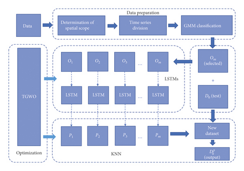
This paper proposes TGWO-LSTM-KNN with the GMM classification model, which includes two parts: data preparation and prediction. GMM is used to choose the input data in the data preparation part considering the spatial-temporal characteristics of freeway traffic flow, while the prediction part is composed of LSTM parallel computing module, KNN module, and TGWO module. The framework of the proposed model is shown in Figure 1.

Details are in the caption following the image — **Figure 1**
Open in figure viewer PowerPoint

Framework of TGWO-LSTM-KNN with GMM classification.

2.1.1. Data Preparation

In the freeway network, the traffic flow of upstream correlates with the prediction point flow, which is considered as spatial correlation. Moreover, the traffic flow of the prediction point changes over time inter- and intraday, and each specific period may have different patterns, such as the morning peak hour and the off-peak hour. Therefore, time series are divided into different parts according to the flow patterns, which will help to improve the accuracy of prediction. The temporal characteristic of prediction point flow is observed through a flow chart. Then set the midpoint of two adjacent extreme points and complete the time series division task.

Related upstream sections are analyzed and selected using GMM binary classification. In this paper, two parameters are used as the classification criteria. One is the KL divergence, which is a commonly used method in information science to quantify the difference between two datasets. In a large-sample traffic dataset with complex distribution, the difference can be simply and quickly reflected. The other is the GRA coefficient, which can analyze the linear similarity between two datasets through a small amount of data. These two parameters can well reflect the correlation of upstream sections and predicted sections. The steps of the classification part are as follows:

Step 1: use time step and speed to determine the space range. Note the upstream points within the scope as O₁ ~ O_m.
Step 2: divide day time into T₁ ~ T_η.
Step 3: construct dataset. Divide the dataset into working days and nonworking days. Change the input time of upstream data to meet the time lag of the prediction point considering the distance and travel speed.
Step 4: calculate the KL divergence and the GRA coefficient in T_i of working days and nonworking days.
Step 5: input the KL divergence and the GRA coefficient into GMM for binary classification. O₁ ~ O_m are divided into two groups in each T_i. The group of points with the KL divergence close to 0 and the GRA coefficient close to 1 is used as the strongly related section of the prediction point for the next prediction.

2.1.2. Prediction

The prediction part consists of three modules, which are LSTM module, KNN module, and TGWO module. KNN is selected at the bottom of the model considering the spatial features of freeway flow with the advantages of fast calculation speed and no lag. LSTM is used to predict the short-term traffic flow of upstream sections and then put the prediction results of upstream sections into KNN to predict the prediction point traffic flow. Because the relationship among upstream points is ignored in the model, multithread LSTM parallel computing (LSTMs) is used to reduce the time consumption of prediction. Also, to improve the performance of LSTM-KNN, TGWO is used to optimize the parameters of LSTM and KNN.

Step 1: use TGWO to optimize the steps and epochs in LSTM, K value in KNN.
Step 2: multithread LSTM parallel computing is used to reduce calculation by ignoring the relationship among upstream points. Each O_i is input into the corresponding LSTM module and then the output P_i set and D₀ together form a new dataset.
Step 3: input the dataset into the KNN module to predict the traffic flow and output .

2.2. Data Preparation

There are three steps in data preparation: determination of spatial scope, time-series division, and GMM classification.

2.2.1. Determination of Spatial Scope

Since the time step of short-term traffic flow prediction (T_step) is usually less than one hour and the highway speed (V) is limited, the radius range of spatial scope can be calculated:

(1)

The accesses and ramps within the radius of the prediction point centered are selected as upstream points.

2.2.2. Time Series Division

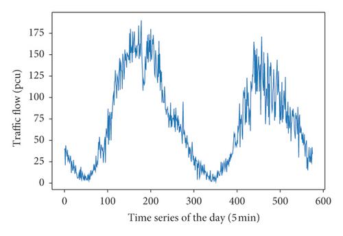
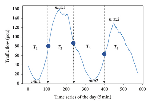
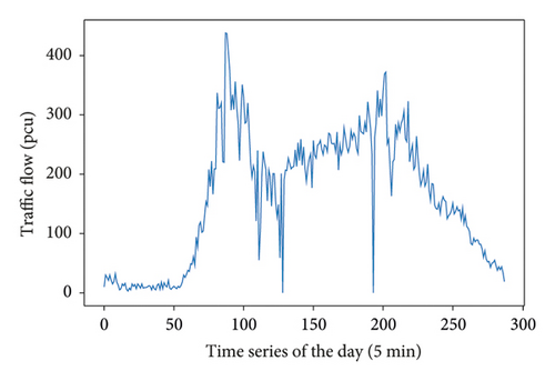
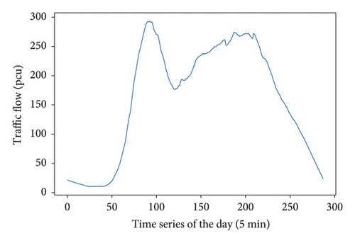
There are random fluctuations in daytime traffic flow, as shown in Figure 2. SG is a method to smooth data based on local least-squares polynomial approximation proposed by Savitzky and Golay [53], which is used to get the extreme traffic value points of the prediction point (D₀) (see Figure 2). Set the point in the middle of the two adjacent extreme values, and each time series between two middle points is a time part (T_i) (see Figure 3).

2.2.3. SG Calculation Method

SG includes two parameters, which are the window length n and the order number k. For the window length n, with the increasing of n, the deviation between the processed data and the real data increases, and also the smoothness. For order number k, with the increasing of k, the deviation between the processed data and the real data decreases, and also the smoothness. According to the characteristics of highway traffic flow and existing research, the choice of n and k in this paper is 31 and 1, respectively.

Input upstream points data O_m = (o_m(1), o_m(2), …, o_m(x)), where x denotes the length of data. Select the window length n and order number k. The data in a window are

. The fitting polynomial is obtained using the k − 1 least square method as follows:

(2)

Then form n equations to form k element equations. If n > k, equation has a solution, then

(3)

The matrix is expressed as

A is the least square fitting solution of different windows, and the value

is as follows:

(4)

Smoothing dataset is

2.2.4. GMM Classification

Gaussian mixture model (GMM) is a probabilistic model that assumes all the data points are generated from a mixture of a finite number of Gaussian distributions with unknown parameters [54], which is used to judge the correlation between upstream and predicted traffic flow, while EM is used to obtain the maximum likelihood estimation of GMM [55]. In this paper, KL-divergence and GRA coefficient are two parameters to do the binary classification.

(1) KL Divergence. KL divergence [56], which is also known as relative entropy, is broadly used as the measurement of the dissimilarity between two probabilistic models [57]. Define KL divergence between O_i = (o_i(1), o_i(2), …, o_i(n)) and D₀ = (d₀(1), d₀(2), …, d₀(n)) as

(5)

The closer KL divergence is to 0, the more similar the two distributions are.

(2) GRA Coefficient. GRA is a method to judge the similarity of different datasets. Compared with traditional Pearson correlation [58], it can use a smaller amount of data to reflect the linear similarity between traffic flows [59]. The steps of GRA are as follows.

Since there is little difference in the magnitude of traffic flow at the same point, the data are initialized by dividing the initial value of the flow o_i(1) and d₀(1).

(6)

where o_i(k) denotes traffic flow of upstream point O₁ in the k time and d_o(k) denotes traffic flow of prediction point D₀ in the k time.

Define the prediction sequence (d₀(1)_GRA, d₀(2)_GRA, …, d₀(n)_GRA) as D_GRA and the factor sequence (o_i(1)_GRA, o_i(2)_GRA, …, o_i(n)_GRA) as. O_iGRA

Then calculate the relation coefficient in the k time

(7)

where ξ denotes the coefficient to control the degree of differentiation, which is generally 0.5 [58].

Define the mean value as GRA coefficient of D₀ and O_i:

(8)

(3) GMM Classification. Let

. GMM is classified by calculating probability. Two-dimensional Gaussian mixture model is as follows:

(9)

where μ_k denotes expectation, Σ_k denotes covariance, n denotes data dimension, ℛ(x|μ_k, Σ_k) denotes k component in a hybrid model, ϑ_k denotes mixture coefficient and

(10)

Then use EM algorithm to calculate ϑ₁, μ₁, Σ₁, ϑ₂, μ₂, Σ₂.

EM-GMM pseudocode is as follows: (Algorithm 1)

Algorithm 1: EM-GMM pseudocode.

function EM − GMM(k⟵2, ϑ₁, μ₁, Σ₁, ϑ₂, μ₂, Σ₂, i⟵0)
do i⟵i + 1:
calculate p(x);
E − step:
until ln pⁱ⁺¹(x|ϑ, μ, Σ) − ln pⁱ(x|ϑ, μ, Σ) < T;
returnϑ₁, μ₁, Σ₁, ϑ₂, μ₂, Σ₂;
end function

2.3. TGWO-LSTM-KNN Hybrid Model

TGWO-LSTM-KNN hybrid model consists of LSTMs module, KNN module, and TGWO module. The specific process is shown in Figure 4.

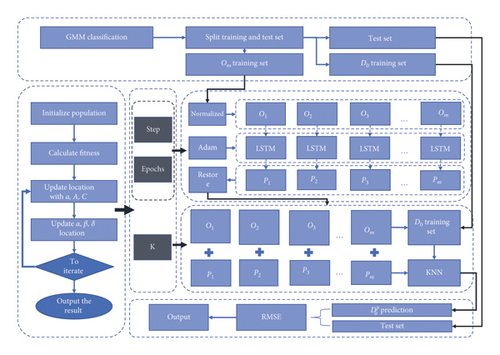
The TGWO-LSTM-KNN model first splits the dataset. The traffic flow of O₁ ~ O_m is trained in the LSTMs module to predict future traffic flow P₁ ~ P_m in parallel. Then use traffic flow dataset consisting of O₁ ~ O_m, P₁ ~ P_m, and D₀ to predict in the KNN module. The step and epochs of LSTM are the parameters with great influence [25], and the coefficient K in the KNN module is also one of the key parameters. Then use the TGWO module to optimize these parameters.

2.3.1. LSTMs Module

LSTM is a special RNN [24] with a forgetting gate. The sigmoid function is used to prevent gradient explosion and disappearance. The traffic flow data of upstream points are trained in different LSTM threads in parallel, which is defined as LSTMs. The data input time is also changed to reduce the lag of the module, which makes LSTM more accurate. The memory unit of the module is shown in Figure 5.

The calculation processes of the memory unit o_m(n) and parameters (see Table 3) are as follows:

(11)

Table 3. LSTM parameters interpretation.

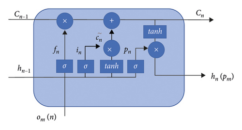
Symbol	Meaning
	The updated state of a memory cell
i_n, f_n, p_n, c_n, h_n	Input gate, forgetting gate, output gate, memory cell, hidden layer output value
w_oc, w_ch	The weight of o_m(n) and the hidden layer
o_m(n)	The input of the n.th data at the m.th upstream point
c_n−1, h_n−1	The output of the memory cell and the hidden layer at n − 1
w_oi, w_hi, w_ci	The weight of the input gate of o_m(n), the hidden layer, and the memory cell
w_of, w_hf, w_cf	The weight of the forgetting gate of o_m(n), the hidden layer, and the memory cell
w_op, w_hp, w_cp	The weight of the output gate of o_m(n), the hidden layer, and the memory cell
b_c, b_i, b_f, b_p	Offset item
tanh and σ	Activation functions
″∘″	Dot product

2.3.2. KNN Module

In this paper, the KNN model is used to predict

by using data of O₁ ~ O_m, P₁ ~ P_m, and D₀. This method not only has high efficiency and less complexity but also can meet the needs of multifactor. Euclidean distance is calculated as follows [14]:

(12)

where d_n denotes the Euclidean distance between P_i in the current time and the O(x) vector x time, P_i denotes the current traffic flow vector of different upstream points (p₁, p₂, …, p_m) in the prediction dataset, p_i denotes the current value of the ith upstream point in P_i, O(x) denotes x time traffic flow vector of different upstream points (o₁(x), o₂(x), …, o_m(x)), o_i(x) denotes the value of ith upstream point in O(x), and m denotes the number of upstream points.

To sort d_x in ascending order, define K smallest O(x) as O(x₁), O(x₂), …, O(x_k) The corresponding values of its prediction point are d₀(x₁), d₀(x₂), …, d₀(x_k). Predict

with weighted method and define prediction set of

at different time as

(13)

where w_i(x_n) denotes weight and

denotes prediction. LSTM-KNN pseudocode is shown in Algorithm 2.

Algorithm 2: LSTM-KNN pseudocode.

function LSTM_KNN(step₁, …, step_n, epochs₁, …, epochs_n, k):
transform dataset into MinMaxScaler(feature_range = (0, 1));
spilt dataset[′O_n′]into O_n trainand O_n test;
LSTMs − step:
thread₁ : look_back⟵step₁; reshape O_1trainand O_1testinto LSTM_datasetwith look_back;
model₁.add(LSTM(n_unit));
model₁.dense(1);
model₁.fit(O_1train, epochs₁, batch_size⟵number of days);
O_1prediction⟵model₁.predict(O_1test);
return O_1prediction;
⋮
thread_n : look_back⟵step_n; reshape O_n train and O_n test into LSTM_dataset with look_back;
model_n.add(LSTM(n_unit));
model_n.dense(1);
model_n.fit(O_n train, epochs_n, batch_size⟵number of days);
O_1prediction⟵model₁.predict(O_1test);
return O_{n prediction};
KNN − step:
knn_test⟵stack O_1prediction, …, O_{n prediction} in sequence horizontally;
knn_train⟵dataset;
knn.fit(knn_train[′O_n′], knn_train[′D₀′]);
knn_prediction⟵knn.predict(knn_test, k);
restore knn_prediction;
return knn_prediction;
end function

The number of units in the hidden layer is n_unit, and the data dimension D of LSTM in each thread is 1, so the time complexity is . On account of the parallel calculation structure, the total time does not change too much with the increasing number of threads. Compared with the original complexity , which reduces a lot of computation and improves efficiency. The time complexity of KNN is O(n), which is only related to the number of data, so the calculation speed is fast.

LSTM has good robustness in traffic prediction [60] and also improves performance by setting reasonable time lag [61] or forgetting layer. KNN can avoid large deviation directly because it calculates the closest Euclidean distance to produce the prediction [62]. These two positive aspects of robustness will support the proposed method to gain more adaptability on data fluctuations and environmental change.

2.3.3. TGWO Module

Grey wolves algorithm was put forward by scholars Mir Jalili Australia in 2014, the Grey wolf groups according to social relations are divided into four grades. Each wolf represents a candidate solution, while the most optimal solution is α_T, the suboptimal solution is β_T, the third optimal solution is δ_T, and the last is ω_T. In each iteration, the three optimum solutions as α_T, β_T, δ_T determine the prey position and direct the ω_T to update the position around it [63].

By using the improved adaptive convergence factor [64], the extremum can be quickly found when the step size is large in a global search. Besides, the extremum can be prevented from missing when the step size becomes smaller in the local search. The weight step size formula [64] adds the weight decreasing strategy, which can reduce unnecessary iterative processes and improve efficiency. The calculation method is as follows.

(1) Initialize the Population. The upper bound U_b and lower bound L_b are defined, respectively. The number of wolves is N. The dimensions are S. M_N×S denotes an N × S two-dimensional matrix, which is the searching field. There are 2m + 1 key parameters to be optimized in each element of the field array, which are step, epochs in the LSTMs module, and the K value in the KNN module. Generate integers randomly at their respective upper and lower bounds to form an element of field array:

(14)

Each parameter has a different U_b and L_b. Set up two vectors to record the bounds.

(15)

(2) Calculate Fitness. Input the element corresponding to each wolf into LSTM-KNN and compare the error. Define the optimal solution as α_T, β_T, δ_T, respectively.

(3) Update location with a_T, A_T, C_T:

(16)

where D denotes the distance between the grey wolves and their prey, t denotes current iteration times, W_P(t) denotes the position of the grey wolf in t iteration times, W(t) denotes the position of the prey in t iteration times, A and C denote the coefficient vectors, r₁ and r₂ denote random coefficients with scalars between 0 and 1, generally take 0.5, a denotes the convergence factor, φ denotes the weight of inertia, φ_max denotes the maximum weight of inertia, generally take 0.9, and φ_min denotes the minimum weight of inertia, generally take 0.4.

(4) Complete the Iteration and Output the Result. The optimal solution α_T is denoted as M_best. The global optimal solution is as follows:

(17)

3. Experiments and Analysis

3.1. Experimental Data

Whitemud Drive is an in-city highway across Edmonton, Alberta, Canada. It is 28 kilometers long with a basic speed limit of 80 kilometers per hour. As a test road, Whitemud Drive is equipped with seven traffic video cameras and seven loop detectors (VDS1017, VDS1037, VDS1034, VDS1031, VDS1029, VDS1027, and VDS1019) from west to east on the main road and gate road to observe the vehicle flow, the vehicle speed, and the vehicle density. In this paper, data of 15 working days are used as historical data for experiments.

3.2. GMM Selecting Test

VDS1019 is set as the prediction point D₀, and the change of traffic flow within one day of the working day is plotted according to 5 mins (see Figure 6). To better carry out the time-division work, the data are smoothed by SG, and the image is reconstructed (see Figure 7).

Find the extreme values, set up the midpoints, and divide the time series (see Figure 8).

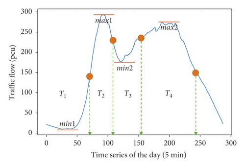
The time-division results are shown in Table 4.

Table 4. Time-division results.

Time part name	Number of data	Time
T₁	0–70	0 : 00–7 : 00
T₂	71–110	7 : 00–9 : 00
T₃	111–155	9 : 00–13 : 00
T₄	156–249	13 : 00–20 : 00

3.2.1. Reconstructing the Dataset by Time-Division

VDS1017, VDS1037, VDS1034, VDS1031, VDS1029, and VDS1027 are recorded as O₁ ~ O₆, their historical data on working days are divided into parts according to T1 ∼ T4, and the data in the same time part are put into the same column. Since the length of the road is 28 km and the speed limit is 80 km/h, we choose 60 km/h as the test speed. It takes 30 mins to go from VDS1017 to VDS1019. Considering the continuity of the road network, the vehicle passes through each point every 5 mins, so O₂ ~ O₆ is delayed by 5–25 mins for input. And the prediction point D₀ is delayed by 30 mins for input. In this way, the data of each day are the delayed input to form a dataset.

Calculate KL divergence and GRA coefficient (see Table 5).

Table 5. Calculation results of KL divergence and GRA coefficient.

KL/GRA result	T1		T2		T3		T4
KL/GRA result	KL	GRA	KL	GRA	KL	GRA	KL	GRA
O₁	0.030	0.90	0.023	0.78	0.020	0.86	0.010	0.87
O₂	0.029	0.90	0.009	0.81	0.017	0.88	0.012	0.86
O₃	0.038	0.89	0.021	0.78	0.031	0.85	0.035	0.82
O₄	0.035	0.90	0.009	0.81	0.018	0.88	0.011	0.85
O₅	0.027	0.91	0.008	0.83	0.016	0.89	0.009	0.87
O₆	0.008	0.95	0.005	0.88	0.004	0.93	0.004	0.92
D	0	1	0	1	0	1	0	1

Input the result table into the GMM module for classification.

Taking T2 as an example, the GMM classification results are shown in Figure 9.

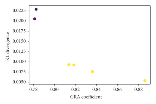
The classification results are two types. The closer the GRA coefficient is to 1, the better the correlation is, and the closer the KL divergence is to 0, the more similar the distribution is. So, choose the yellow mark points as the input points (see Figure 9). The following is the final classification results of four datasets (see Table 6).

Table 6. Classification results of GMM.

GMM result	T1	T2	T3	T4
D point	O₆	O₂, O₄, O₅, O₆	O₂, O₄, O₅, O₆	O₁, O₂, O₄, O₅, O₆

The upstream points selected between T2 and T3 are the same, so T2 and T3 can be regarded as the same time part, which is 7 : 00–13 : 00, and the dataset T₂₊₃ can be reconstructed. The next experimental data are T₂₊₃.

3.3. Comparative Experiments at Different Upstream Points

Different upstream points are selected for model prediction and mean absolute percentage error (MAPE) comparison so as to verify the effect after classification. Results are shown in Table 7.

Table 7. MAPE comparison table of different points.

Model/points	V34	V34 + V31	V34 + V31 + V29	V34 + V31 + V29 + V27	Including abandonment points
LSTM-KNN	14.45	14.96	14.31	12.19	12.46
Linear-SVM	20.47	21.14	20.03	21.17	21.24
Poly-SVM	15.85	17.30	17.15	17.65	18.04
RBF-SVM	20.51	20.29	20.87	20.17	20.48
Multi-LSTM	14.32	14.51	11.96	9.51	23.14

In this dataset, it can be seen that the abandoned upstream points have little difference from the selected points (see Table 5). So it is not obvious in the accuracy improvement, which is reasonable. If in datasets with a large difference, the meaning of GMM classification operation will be reflected more.

3.4. TGWO-LSTM-KNN Experiments

3.4.1. LSTM-KNN Structural Test

Considering the operation time and efficiency, this paper constructs the following structures for testing. Since the training data are 15 days’ traffic flow, the batch size is set to 15, and the data are divided into 15 groups, which will ignore the data relationship between each group and reduce the risk of overfitting. If the batch size is too small, it is not conducive to the training model and is easy to overfitting. The test step is 3, epochs are 100, and the comparison results are shown in Table 8.

Table 8. Error comparison table of different structures.

Structure	RMSE	MAE	MAPE
Double-layer structure	42.49	29.81	11.64
LSTM (256 units) +
LSTM (128 units)

Four-layer structure	44.87	31.33	12.25
LSTM (256 units) +
Dropout (0.2) +
LSTM (128 units) +
Dropout (0.2)

Single-layer structure	44.42	31.55	12.32
LSTM (256 units)	44.42	31.55	12.32

Single-layer structure	44.43	31.29	12.19
LSTM (128 units)	44.43	31.29	12.19

The results show that increasing the number of LSTM layers can improve the prediction accuracy, but it increases a lot of computing time and overfits easily. Increasing the forgetting layer (the forgetting rate is 0.2) will reduce the accuracy. In the first-layer structure, there is only a small difference between 256 units and 128 units; therefore, the single-layer 128 units structure is selected for prediction in the following LSTM.

3.4.2. LSTM-KNN Time Steps Test

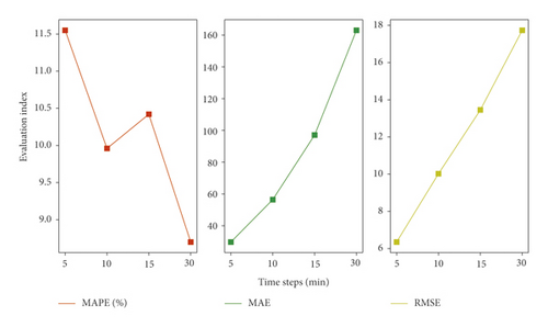
The model is tested under different time steps (5 mins, 10 mins, 15 mins, and 30 mins). The result shows that the model has good accuracy and stability (see Figure 10). The overall prediction accuracy shows a downward trend, and the absolute error shows an upward trend. It is worth noting that when the time step is 10 mins, the trend of accuracy will change and the error is lower than 15 mins. In general, even if the time step is different, the model still has good performance for the prediction accuracy.

3.4.3. TGWO Optimization Test

The dataset has four upstream points, and the key parameters to be optimized are the steps of O₂, O₄, O₅, O₆, the training epochs in the LSTM module, and the K in the KNN module. So, M_{[i, j]} = [step₂, step₄, step₅, step₆, epochs₂, epochs₄, epochs₅, epochs₆, k]. Set the upper and lower bounds: the step size ranges from 3 to 20. Training time ranges from 100 to 200. The coefficient K ranges from 5 to 50, the number of iterations t is 50, the number of wolves is N = 5, and the dimension S is 30. The training results are shown in Figure 11.

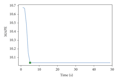
When the MAPE is 10.04 (green mark in Figure 11), it will reach the optimal solution M_best = [5,6,5,6,120,100, 120,100,25]. The steps of O₂, O₅ and O₄, O₆ are 5 and 6, the training epochs are 120 and 100, and K is 25.

3.4.4. Comparison of TGWO-LSTM-KNN and Other Models

TGWO-LSTM-KNN is compared with SVM, LSTM, and BP. The parameters of TGWO-LSTM-KNN are the optimal solution. The step of LSTM-KNN is 3, K is 16, and the epochs is 100. LSTM has 256 units in the first layer and 128 units in the second layer of the double-hidden layer structure, with the step of 3 and epochs of 100. SVM uses three modes to fit, linear and poly, RBF. BP neural network is a three-layer structure, two fully connected layers, the middle increased the forgetting layer (rate is 0.2), and the epochs is 100. Results are shown in Figure 12.

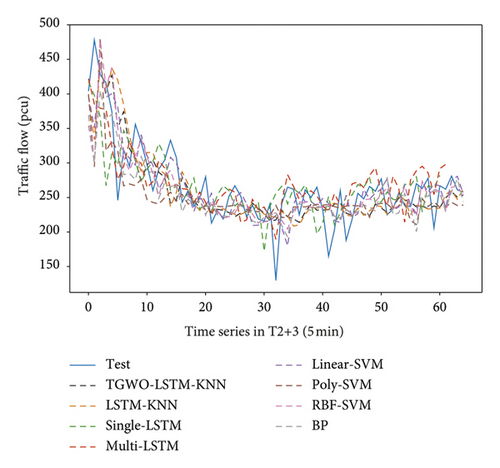
The accuracy of LSTM-KNN can reach the level of the popular model. The accuracy of TGWO-LSTM-KNN can be improved by 15.27% compared with single-LSTM, 9.47% compared with BP, and 43.12% compared with poly-SVM (see Table 9). Besides, the advantage of the hybrid model is not accuracy, but being able to output the prediction set of upstream points for collaborative management.

Table 9. Error comparison table of different models.

Model	RMSE	MAE	MAPE
TGWO-LSTM-KNN	29.70	23.17	10.04
LSTM-KNN	44.43	31.29	12.19
Single-LSTM	36.75	27.88	11.85
Multi-LSTM	33.32	24.52	9.51
BP	37.59	27.59	11.09
Linear-SVM	38.78	27.03	21.17
Poly-SVM	45.36	33.87	17.65
RBF-SVM	40.62	28.29	20.17

4. Conclusions

In this paper, the TGWO-LSTM-KNN prediction model with GMM classification considering spatial-temporal characteristics under the concept of attention mechanism is proposed. The time series is divided into parts by using the temporal characteristic of the prediction point. And GMM through KL and GRA is used for further classification. The upstream points with a small difference in distribution and high linear similarity are selected to increase the accuracy and reduce the complexity. Then the hybrid model TGWO-LSTM-KNN is used to train and predict. Parallel computing is used in the LSTM module to improve efficiency.

GMM as an unsupervised model can be very flexible to classify. This model can be applied to the multifactor model to reduce complexity. KNN, as the next part of LSTM, fully combines upstream points data and prediction points data for prediction. Compared with SVM, KNN has the characteristics of fast speed and greater data processing ability, which is more suitable for multiple factors and complex data of freeway. LSTMs module can ignore the relationship between upstream points to perform the parallel computation. It can reduce the operation time and make the model more practical. TGWO is less likely to fall into local optimal solution and also has fast speed and good performance. To sum up, TGWO-LSTM-KNN with GMM classification can be better used in real freeways with complex data and multifactor with high accuracy, fast calculation speed, and strong adaptability. It can be applied in the real freeway to achieve the purpose of collaborative management.

Conflicts of Interest

The authors declare that they have no conflicts of interest.

Acknowledgments

The authors want to thank Tianjiao Wang, Xi Chen, Xiang Wang, and Lingbin Kong for their help in the study. Thanks also should be given to the OpenITS platform (http://www.openits.cn/). The research and publication of this article were funded by the National Natural Science Foundation of China (52072129).

Open Research

Data Availability

The data used to support the findings of this study are openly available in the OpenITS platform for noncommercial purposes only and the website is https://www.openits.cn/openData1/700.jhtml.

References

1 Qi C. and Hou Z.-S., Application of adaptive single-exponent smoothing for short-term traffic flow prediction, Control Theory & Applications. (2012) 29, no. 4, 465–469.
Google Scholar
2 Chan K. Y., Dillon T. S., Singh J., and Chang E., Neural-network-based models for short-term traffic flow forecasting using a hybrid exponential smoothing and levenberg-marquardt algorithm, IEEE Transactions on Intelligent Transportation Systems. (2012) 13, no. 2, 644–654, https://doi.org/10.1109/tits.2011.2174051, 2-s2.0-84861893114.
10.1109/TITS.2011.2174051
Web of Science® Google Scholar
3 Gao H. and Zhang D., Traffic flow forecasting model based on fractal and three-exponential smoothing, Journal of Nanjing University of Posts and Telecommunications (Natural Science Edition). (2018) 38, no. 6, 63–67.
Google Scholar
4 Lv L., Chen M., Liu Y., and Yu X., T. Cao, E. P. Lim, Z. H. Zhou, T. B. Ho, D. Cheung, and H. Motoda, A plane moving average algorithm for short-term traffic flow prediction, Advances in Knowledge Discovery and Data Mining, 2015, Springer, Cham, Switzerland, 357–369, https://doi.org/10.1007/978-3-319-18032-8_28, 2-s2.0-84945572691.
10.1007/978-3-319-18032-8_28
Google Scholar
5 Mai T., Ghosh B., and Wilson S., Short-term traffic-flow forecasting with auto-regressive moving average models, Proceedings of the Institution of Civil Engineers - Transport. (2014) 167, no. 4, 232–239, https://doi.org/10.1680/tran.12.00012, 2-s2.0-84931055524.
10.1680/tran.12.00012
Web of Science® Google Scholar
6 Billings D. and Jiann-Shiou Y., Application of the ARIMA models to urban roadway travel time prediction - a case study, 1-6, Proceedings of the 2006 IEEE International Conference on Systems, Man and Cybernetics, October 2006, Toronto, ON, Canada, https://doi.org/10.1109/icsmc.2006.385244, 2-s2.0-34548134136.
10.1109/icsmc.2006.385244
Google Scholar
7 Kumar S. V. and Vanajakshi L., Short-term traffic flow prediction using seasonal ARIMA model with limited input data, European Transport Research Review. (2015) 7, no. 3, https://doi.org/10.1007/s12544-015-0170-8, 2-s2.0-84931263119.
10.1007/s12544-015-0170-8
Web of Science® Google Scholar
8 Liu J. and Guan W., A summary of traffic flow forecasting methods, Journal of Highway and Transportation Research and Development. (2004) 3, 82–85.
Google Scholar
9 Guo J., Huang W., and Williams B. M., Adaptive Kalman filter approach for stochastic short-term traffic flow rate prediction and uncertainty quantification, Transportation Research Part C: Emerging Technologies. (2014) 43, 50–64, https://doi.org/10.1016/j.trc.2014.02.006, 2-s2.0-84902553625.
10.1016/j.trc.2014.02.006
Web of Science® Google Scholar
10 Ojeda L. L., Kibangou A. Y., and De Wit C. C., Adaptive kalman filtering for multi-step ahead traffic flow prediction, Proceedings of the 2013 American Control Conference, June 2013, Washington, DC, USA, 4724–4729.
Google Scholar
11 Liyan Z., Jian M., and Jian S., Examples of validating an adaptive kalman filter model for short-term traffic flow prediction, Proceedings of the Twelfth COTA International Conference of Transportation Professionals, December 2012, Xi’an, China.
Google Scholar
12 Zhou T., Jiang D., Lin Z., Han G., Xu X., and Qin J., Hybrid dual Kalman filtering model for short-term traffic flow forecasting, IET Intelligent Transport Systems. (2019) 13, no. 6, 1023–1032, https://doi.org/10.1049/iet-its.2018.5385, 2-s2.0-85067070063.
10.1049/iet-its.2018.5385
Web of Science® Google Scholar
13 Zhang S., Song Y., Jiang D., Zhou T., and Qin J., Noise-identified kalman filter for short-term traffic flow forecasting, Proceedings of the 2019 15th International Conference on Mobile Ad-Hoc and Sensor Networks (MSN), Decmber 2019, Shenzhen, China.
Google Scholar
14 Zhang L., Liu Q., Yang W., Wei N., and Dong D., An improved K-nearest neighbor model for short-term traffic flow prediction, Procedia - Social and Behavioral Sciences. (2013) 96, 653–662, https://doi.org/10.1016/j.sbspro.2013.08.076.
10.1016/j.sbspro.2013.08.076
Web of Science® Google Scholar
15 Zheng W., Lee D.-H., and Shi Q., Short-term freeway traffic flow prediction: Bayesian combined neural network approach, Journal of Transportation Engineering. (2006) 132, no. 2, 114–121, https://doi.org/10.1061/(asce)0733-947x(2006)132:2(114), 2-s2.0-31044437283.
10.1061/(ASCE)0733-947X(2006)132:2(114)
Web of Science® Google Scholar
16 Zhang Y. and Xie Y., Forecasting of short-term freeway volume with v-support vector machines, Transportation Research Record: Journal of the Transportation Research Board. (2007) 2024, no. 1, 92–99, https://doi.org/10.3141/2024-11, 2-s2.0-40449104106.
10.3141/2024-11
Web of Science® Google Scholar
17 Sun Y., Leng B., and Guan W., A novel wavelet-SVM short-time passenger flow prediction in Beijing subway system, Neurocomputing. (2015) 166, 109–121, https://doi.org/10.1016/j.neucom.2015.03.085, 2-s2.0-84931575772.
10.1016/j.neucom.2015.03.085
Web of Science® Google Scholar
18 Min D., Short-time prediction of traffic flow based on PSO optimized SVM, Proceedings of the 2018 International Conference on Intelligent Transportation, Big Data & Smart City (ICITBS), January 2018, Xiamen, China.
Google Scholar
19 Smith B. L. and Demetsky M. J., Short-term traffic flow prediction models-a comparison of neural network and nonparametric regression approaches, Proceedings of the Proceedings of IEEE International Conference on Systems, Man and Cybernetics, October 1994, Bari, Italy.
Google Scholar
20 Dehuri S. and Cho S.-B., A comprehensive survey on functional link neural networks and an adaptive PSO-BP learning for CFLNN, Neural Computing & Applications. (2010) 19, no. 2, 187–205, https://doi.org/10.1007/s00521-009-0288-5, 2-s2.0-80054727848.
10.1007/s00521-009-0288-5
Web of Science® Google Scholar
21 Wang S., Zhang N., Wu L., and Wang Y., Wind speed forecasting based on the hybrid ensemble empirical mode decomposition and GA-BP neural network method, Renewable Energy. (2016) 94, 629–636, https://doi.org/10.1016/j.renene.2016.03.103, 2-s2.0-84962148959.
10.1016/j.renene.2016.03.103
Web of Science® Google Scholar
22 Vincent P., Larochelle H., Lajoie I., Bengio Y., and Manzagol P.-A., Stacked denoising autoencoders: learning useful representations in a deep network with a local denoising criterion, Journal of Machine Learning Research. (2010) 11, 3371–3408.
Web of Science® Google Scholar
23 Gers F. A., Schmidhuber J., and Cummins F., Learning to forget: continual prediction with LSTM, Neural Computation. (2000) 12, no. 10, 2451–2471, https://doi.org/10.1162/089976600300015015, 2-s2.0-0034293152.
10.1162/089976600300015015
CAS PubMed Web of Science® Google Scholar
24 Hochreiter S. and Schmidhuber J., Long short-term memory, Neural Computation. (1997) 9, no. 8, 1735–1780, https://doi.org/10.1162/neco.1997.9.8.1735, 2-s2.0-0031573117.
10.1162/neco.1997.9.8.1735
CAS PubMed Web of Science® Google Scholar
25 Gers F. A., Schraudolph N. N., and Schmidhuber J., Learning precise timing with LSTM recurrent networks, Journal of Machine Learning Research. (2003) 3, no. 1, 115–143.
Web of Science® Google Scholar
26 Sundermeyer M., Schlueter R., and Ney H., LSTM Neural Networks for Language Modeling, 2012, Interspeech 2012, Portland, OR, USA.
10.21437/Interspeech.2012-65
Google Scholar
27 Zhou C., Sun C., Liu Z., and Lau F. C. M., A C-LSTM neural network for text classification, Computer Science. (2015) 1, no. 4, 39–44.
Google Scholar
28 Graves A. and Schmidhuber J., Framewise phoneme classification with bidirectional LSTM and other neural network architectures, Neural Networks. (2005) 18, no. 5-6, 602–610, https://doi.org/10.1016/j.neunet.2005.06.042, 2-s2.0-27744588611.
10.1016/j.neunet.2005.06.042
PubMed Web of Science® Google Scholar
29 Fu R., Zhang Z., and Li L., Using LSTM and GRU neural network methods for traffic flow prediction, Proceedings of the 2016 31st Youth Academic Annual Conference of Chinese Association of Automation (YAC), November 2016, Wuhan, China.
Google Scholar
30 Kong W., Dong Z. Y., Jia Y., Hill D. J., Xu Y., and Zhang Y., Short-term residential load forecasting based on LSTM recurrent neural network, Ieee Transactions on Smart Grid. (2019) 10, no. 1, 841–851, https://doi.org/10.1109/tsg.2017.2753802, 2-s2.0-85030636120.
10.1109/TSG.2017.2753802
Web of Science® Google Scholar
31 Alahi A., Goel K., Ramanathan V., Robicquet A., Fei-Fei L., and Savarese S., Social LSTM: human trajectory prediction in crowded spaces, Proceedings of the 2016 Ieee Conference on Computer Vision and Pattern Recognition, June 2016, Las Vegas, NV, USA, 961–971, https://doi.org/10.1109/cvpr.2016.110, 2-s2.0-84986253439.
10.1109/cvpr.2016.110
Google Scholar
32 Sak H., Senior A., and Beaufays F., Long short-term memory recurrent neural network architectures for large scale Acoustic modeling, Proceedings of the 15th Annual Conference of the International Speech Communication Association, September 2014, Graz, Austria, 338–342, https://doi.org/10.21437/interspeech.2014-80.
10.21437/interspeech.2014-80
Google Scholar
33 Wen H., Zhang D., and Siuyan L., Application of GA-LSTM model in highway traffic flow prediction, Journal of Harbin Institute of Technology. (2019) 51, no. 9, 81–87+95.
Google Scholar
34 Tu J. V., Advantages and disadvantages of using artificial neural networks versus logistic regression for predicting medical outcomes, Journal of Clinical Epidemiology. (1996) 49, no. 11, 1225–1231, https://doi.org/10.1016/s0895-4356(96)00002-9, 2-s2.0-0030297904.
10.1016/S0895-4356(96)00002-9
CAS PubMed Web of Science® Google Scholar
35 Guo J., Liu Y., and Ma L., Assignee. EEMD-IAGA-BP Neural Network Based Ship Traffic Flow Predicting Method, Involves Constructing Three-Layer BP Neural Network with Enhanced Adaptive Genetic Algorithm Optimization as Training Model, and Obtaining Predicted Results Patent CN110111606-A, 2021, Inventors; Univ Shanghai Maritime, Shanghai Shi, China.
Google Scholar
36 Liong S. Y. and Sivapragasam C., Flood stage forecasting with support vector machines, Journal of the American Water Resources Association. (2002) 38, no. 1, 173–186, https://doi.org/10.1111/j.1752-1688.2002.tb01544.x, 2-s2.0-0036202123.
10.1111/j.1752-1688.2002.tb01544.x
Web of Science® Google Scholar
37 Duo M., Qi Y., Lina G., and Xu E., A short-term traffic flow prediction model based on EMD and GPSO-SVM, Proceedings of the 2017 IEEE 2nd Advanced Information Technology, Electronic and Automation Control Conference (IAEAC), March 2017, Chongqing, China.
Google Scholar
38 Chung H. and andShin K.-s, Genetic algorithm-optimized long short-term memory network for stock market prediction, Sustainability. (2018) 10, no. 10, https://doi.org/10.3390/su10103765, 2-s2.0-85055111230.
10.3390/su10103765
Web of Science® Google Scholar
39 Zhou W. and Meng S., Assignee. Navigation Reminder Method Based on SVD-PSO-LSTM for Predicting Short-Term Traffic Flow, Involves Providing First Train and Optimizes LSTM Model, Then Collects Historical Traffic Flow Data, and Preprocesses and Input to Training Flow Data Patent CN111709549-A, 2021, Inventors; Univ Donghua, Shanghai, China.
Google Scholar
40 Luo X., Li D., Yang Y., and Zhang S., Spatiotemporal traffic flow prediction with KNN and LSTM, Journal of Advanced Transportation. (2019) 2019, 10, https://doi.org/10.1155/2019/4145353, 2-s2.0-85062797127.
10.1155/2019/4145353
Google Scholar
41 Dai L., Mei H., Qian C., Yun M., and Jin-Ming L., Survey on short-term traffic flow forecasting based on deep learning, Computer Science. (2019) 46, no. 3, 39–47.
Google Scholar
42 Su F., Dong H., Jia L., Tian Z., and Sun X., Space-time correlation analysis of traffic flow on road network, International Journal of Modern Physics B. (2017) 31, no. 5, https://doi.org/10.1142/s0217979217500278, 2-s2.0-84997047793.
10.1142/S0217979217500278
PubMed Web of Science® Google Scholar
43 Liu Q., Cai Y., Jiang H., Chen X., and Lu J., Traffic state spatial-temporal characteristic analysis and short-term forecasting based on manifold similarity, Ieee Access. (2018) 6, 9690–9702, https://doi.org/10.1109/access.2017.2788639, 2-s2.0-85040035733.
10.1109/ACCESS.2017.2788639
Web of Science® Google Scholar
44 Wang C., Attention-based traffic flow prediction and research, 2020, East China Jiaotong University, Nanchang, China, Degree Diss.
Google Scholar
45 LI L., Research on spatial temporal prediction model of traffic flow based on attentional mechanism, 2020, South China University of Technology, Guangzhou, China, Degree Diss.
Google Scholar
46 Chen M., Research on traffic flow prediction based on improved graph attention network, 2021, Shanghai Normal University, Shanghai, China, Degree Diss.
Google Scholar
47 Ma D., Song X. B., Zhu J., and Ma W., Input data selection for daily traffic flow forecasting through contextual mining and intra-day pattern recognition, Expert Systems with Applications. (2021) 176, https://doi.org/10.1016/j.eswa.2021.114902.
10.1016/j.eswa.2021.114902
Web of Science® Google Scholar
48 Ma D., Song X., and Li P., Daily traffic flow forecasting through a contextual convolutional recurrent neural network modeling inter- and intra-day traffic patterns, IEEE Transactions on Intelligent Transportation Systems. (2021) 22, no. 5, 2627–2636, https://doi.org/10.1109/tits.2020.2973279.
10.1109/TITS.2020.2973279
Web of Science® Google Scholar
49 Qu L., Li W., Li W., Ma D., and Wang Y., Daily long-term traffic flow forecasting based on a deep neural network, Expert Systems with Applications. (2019) 121, 304–312, https://doi.org/10.1016/j.eswa.2018.12.031, 2-s2.0-85058786761.
10.1016/j.eswa.2018.12.031
Web of Science® Google Scholar
50 Song X., Li W., Ma D., Wang D., Qu L., and Wang Y., A match-then-predict method for daily traffic flow forecasting based on group method of data handling, Computer-Aided Civil and Infrastructure Engineering. (2018) 33, no. 11, 982–998, https://doi.org/10.1111/mice.12381, 2-s2.0-85054599576.
10.1111/mice.12381
Web of Science® Google Scholar
51 Ma D., Sheng B., Ma X., and Jin S., Fuzzy hybrid framework with dynamic weights for short-term traffic flow prediction by mining spatio-temporal correlations, IET Intelligent Transport Systems. (2020) 14, no. 2, 73–81, https://doi.org/10.1049/iet-its.2019.0287.
10.1049/iet-its.2019.0287
Web of Science® Google Scholar
52 Hao S., Lee D.-H., and Zhao D., Sequence to sequence learning with attention mechanism for short-term passenger flow prediction in large-scale metro system, Transportation Research Part C: Emerging Technologies. (2019) 107, 287–300, https://doi.org/10.1016/j.trc.2019.08.005, 2-s2.0-85071139877.
10.1016/j.trc.2019.08.005
Web of Science® Google Scholar
53 Steinier J., Termonia Y., and Deltour J., Smoothing and differentiation of data by simplified least square procedure, Analytical Chemistry. (1972) 44, no. 11, 1906–1909, https://doi.org/10.1021/ac60319a045, 2-s2.0-0345591924.
10.1021/ac60319a045
CAS PubMed Web of Science® Google Scholar
54 Reynolds D., Gaussian Mixture Models, 2008, Springer US, Berlin, Germany.
Google Scholar
55 Bilmes J. A., A gentle tutorial of the EM algorithm and its application to parameter estimation for Gaussian mixture and hidden Markov models, International Computer Science Institute. (1998) 4, no. 510.
Google Scholar
56 Kullback S. and Leibler R. A., On information and sufficiency, The Annals of Mathematical Statistics. (1951) 22, no. 1, 79–86, https://doi.org/10.1214/aoms/1177729694.
10.1214/aoms/1177729694
Web of Science® Google Scholar
57 Liu S., Wen Z., Tao J. et al., A data driven method for target and concatenation cost calculation with KL-divergence in Mandarin hybrid speech synthesis, Proceedings of the 2014 12th International Conference on Signal Processing, October 2014, HangZhou, China, 572–576, https://doi.org/10.1109/icosp.2014.7015069, 2-s2.0-84988248546.
10.1109/icosp.2014.7015069
Google Scholar
58 Gerhard N., Pearson Correlation Coefficient, 2009, Springer, Vienna, Austria, https://doi.org/10.1007/978-3-211-89836-9.
Google Scholar
59 Deng J., Introduction to grey system theory, Journal of Grey System. (1989) 1, no. 1, 1–24.
Google Scholar
60 Wang X., Xu L., and Chen K., Data-driven short-term forecasting for urban road network traffic based on data processing and LSTM-RNN, Arabian Journal for Science and Engineering. (2019) 44, no. 4, 3043–3060.
10.1007/s13369-018-3390-0
Web of Science® Google Scholar
61 Sangiorgio M. and Dercole F., Robustness of LSTM neural networks for multi-step forecasting of chaotic time series, Chaos Solitons & Fractals. (2020) 139, https://doi.org/10.1016/j.chaos.2020.110045.
10.1016/j.chaos.2020.110045
Web of Science® Google Scholar
62 Habtemichael F. G. and Cetin M., Short-term traffic flow rate forecasting based on identifying similar traffic patterns, Transportation Research Part C: Emerging Technologies. (2016) 66, 61–78, https://doi.org/10.1016/j.trc.2015.08.017, 2-s2.0-84941585169.
10.1016/j.trc.2015.08.017
Web of Science® Google Scholar
63 Mirjalili S., Mirjalili S. M., and Lewis A., Grey wolf optimizer, Advances in Engineering Software. (2014) 69, 46–61.
10.1016/j.advengsoft.2013.12.007
Web of Science® Google Scholar
64 Zhang W. S., Hao Z. Q, Zhu J. J., Du T. T., and Hao H. M., BP neural network model for short-time traffic flow forecasting based on transformed grey wolf optimizer algorithm, Journal of Transportation Systems Engineering & Information Technology. (2020) 20, no. 02, 196–203.
Google Scholar

Citing Literature

All articles

Short-Term Traffic Prediction considering Spatial-Temporal Characteristics of Freeway Flow

Abstract

1. Introduction

2. Methodology

2.1. Framework

2.1.1. Data Preparation

2.1.2. Prediction

2.2. Data Preparation

2.2.1. Determination of Spatial Scope

2.2.2. Time Series Division

2.2.3. SG Calculation Method

2.2.4. GMM Classification

2.3. TGWO-LSTM-KNN Hybrid Model

2.3.1. LSTMs Module

2.3.2. KNN Module

2.3.3. TGWO Module

3. Experiments and Analysis

3.1. Experimental Data

3.2. GMM Selecting Test

3.2.1. Reconstructing the Dataset by Time-Division

3.3. Comparative Experiments at Different Upstream Points

3.4. TGWO-LSTM-KNN Experiments

3.4.1. LSTM-KNN Structural Test

3.4.2. LSTM-KNN Time Steps Test

3.4.3. TGWO Optimization Test

3.4.4. Comparison of TGWO-LSTM-KNN and Other Models

4. Conclusions

Conflicts of Interest

Acknowledgments

Open Research

Data Availability

References

Citing Literature

Figures

References

Information

About Wiley Online Library

Help & Support

Opportunities

Connect with Wiley