In recent years, Differential Evolution (DE) has shown excellent performance in solving optimization problems over continuous space and has been widely used in many fields of science and engineering. How to avoid the local optimal solution and how to improve the convergence performance of DE are hotpot problems for many researchers. In this paper, an improved differential evolution algorithm based on dual-strategy (DSIDE) is proposed. The DSIDE algorithm has two strategies. (1) An enhanced mutation strategy based on “DE/rand/1,” which takes into account the influence of reference individuals on mutation and has strong global exploration and convergence ability. (2) A novel adaptive strategy for scaling factor and crossover probability based on fitness value has a positive impact on population diversity. The DSIDE algorithm is verified with other seven state-of-the-art DE variants under 30 benchmark functions. Furthermore, Wilcoxon sign rank-sum test, Friedman test, and Kruskal–Wallis test are utilized to analyze the results. The experiment results show that the proposed DSIDE algorithm can significantly improve the global optimization performance.

1. Introduction

Differential Evolution (DE) is an emerging optimization technique proposed by Storn and Price [1] in 1995, which was initially used to solve Chebyshev polynomials. Later, it is demonstrated that DE is also an effective method to solve complex optimization problems. Similar to other intelligent evolutionary algorithms, DE is a stochastic parallel optimization algorithm based on swarm intelligence, which guides optimization search by imitating heuristic swarm intelligence generated by cooperation and competition among individuals in the population.

In DE, the population consists of several individuals, each of which representing a potential solution to an optimization problem. DE generates offspring individuals through mutation, crossover, and selection, and the offspring individuals are expected to be closer to the optimal solution. In the process of evolution, with the increase of generations, the population diversity becomes worse, leading to premature convergence or evolutionary stagnation, which is undoubtedly fatal to the algorithm that depends on the difference of population. Also, the performance of DE is affected by control parameters [2, 3]. For different optimization problems, these control parameters often need a large number of repeated experiments to adjust to the appropriate value for achieving better optimization effect.

To address these shortcomings in DE, many improvements have been proposed, most of which focused on control parameters and mutation strategies.

Population size NP, scaling factor F, and crossover probability CR are three crucial control parameters in DE. Experiments in many works of literatures show that the performance of DE can be improved by adjusting these control parameters. Omran et al. [4] proposed a self-adaptation scheme (SDE), in which F was adaptive and CR was generated by a normal distribution. Liu and Lampinen [5] proposed a fuzzy adaptive differential evolution algorithm (FADE), which used the fuzzy logic controller to adjust F, and CR dynamically and successfully evolved individuals and their fitness values as input parameters of the logic controller. Brest et al. [6] developed a new adaptive DE algorithm, named jDE, applying F and CR to the individual level. If a better individual is produced, these parameters would be retained; otherwise, they would be adjusted according to two constants. Noman et al. [7] proposed an adaptive differential evolution algorithm (aDE), which was similar to jDE [6], except that the updating of parameters in aDE depended on whether the offspring was better than the average individual in the parent population. Asafuddoula et al. [8] used roulette to select the suitable CR value for each individual in each generation of the population. Tanabe and Fukunaga [9] proposed the success-history-based parameter adaptation for differential evolution (SHADE), which generated new F and CR pairs by sampling the nearby space of stored parameter pairs. Later, they came up with an improved version called L-SHADE [10]. Based on SHADE, a linear population size reduction strategy (LPSR) was adopted to reduce the population size NP by a linear function continuously. Zhu et al. [11] proposed an adaptive population tuning scheme (APTS) that dynamically adjusted the population size, in which redundant individuals were removed from the population or “excellent” individuals were generated. Zhao et al. [12] proposed a self-adaptive DE with population adjustment scheme (SAPA) to tune the size of the offspring population, which contained two kinds of population adjustment schemes. Pan et al. [13] proposed a parameter adaptive DE algorithm on real-parameter optimization, in which better control parameters F and CR are more likely to survive and produce good offspring. An enhancing DE with novel parameter control, referred to as DE-NPC, was proposed by Meng et al. [14]. The update of F and CR was based on the location information of the population and the success probability of CR, respectively, and a combined parabolic-linear population size reduction scheme was adopted. Di Carlo et al. [15] proposed a multipopulation adaptive version of inflationary DE algorithm (MP-AIDEA), the parameters F and CR of which were adjusted together with the local restart bubble size and the number of local restarts of Monotonic Basin Hopping [16]. Li et al. [17] presented an enhanced adaptive differential evolution algorithm (EJADE), in which CR sorting mechanism and dynamic population reduction strategy were introduced.

To improve the optimization performance and balance the contradiction between global exploration and local exploitation, researchers have carried out a lot of work on mutation strategy in DE. Das et al. [18] proposed an improved algorithm based on “DE/current-to-best/1” strategy, which made full use of the optimal individual information in the neighborhood to guide the mutation operation. Zhang and Sanderson [19] proposed an adaptive differential evolution algorithm (JADE), which adopted “DE/current-to-pbest/1” mutation model, used suboptimal solutions to improve population diversity, and employed Cauchy and Normal distribution to generate F and CR. Qin et al. [20] proposed a self-adaptive DE (SaDE), which adopted four mutation strategies to generate mutation individuals. The selection of mutation strategy would be affected by previous performance. A DE algorithm (CoDE) using three mutation strategies and three parameters for the random combination was presented by Wang et al. [21]. Epitropakis et al. [22] proposed a novel framework that specified the selection probability in the mutation operation based on the distance between each individual and the mutation individual, thereby guiding the population to global optimization. Mallipeddi et al. [23] proposed the EPSDE algorithm, which was characterized by a stochastic selection of mutation strategies and parameters in a candidate pool consisting of three basic mutation strategies and preset parameters. Xiang et al. [24] proposed an enhanced differential evolution algorithm (EDE), which adopted a new combined mutation strategy composed of “DE/current/1” and “DE/pbest/1.” Cui et al. [25] proposed a DE algorithm based on adaptive multiple subgroups (MPADE), which divided the population into three subgroups according to fitness values, each subgroup had its mutation strategy. Wu et al. [26] presented a DE with multipopulation-based ensemble of mutation strategies (MPEDE), which had three mutation strategies, three indicator subgroups, and one reward subgroup. After several evolutionary generations, the reward subgroup was dynamically assigned to the best-performing mutation strategy. Parameters with an adaptive learning mechanism for the enhancement of differential evolution (PALM-DE) were presented by Meng et al. [27]. Unlike the external archive of the mutation strategy in JADE [19] and SHADE [9], the inferior solution archive in PALM-DE mutation strategy used a timestamp mechanism. In [28], Meng et al. introduced a novel parabolic population size reduction scheme and an enhanced timestamp-based mutation strategy to tackle the weakness of previous mutation strategy. Wei et al. [29] proposed the RPMDE algorithm, designed the “DE/M_pbest-best/1” mutation strategy, used the optimal individual group information to generate new solutions, and adopted the random perturbation method to avoid falling into the local optimal. Duan’s DPLDE [30] algorithm used population diversity and population fitness to determine individuals participating in mutation operation, thus influencing the mutation strategy. Tian and Gao [31] proposed NDE, which employed two mutation operators based on neighborhood-based and an individual-based selection probability to adjust the search performance of each individual appropriately. Wang et al. [32] proposed the DE algorithm based on particle swarm optimization (DEPSO), which utilized the improved “DE/rand/1” mutation strategy and PSO mutation strategy. Meng and Pan [33] presented hierarchical archive based on mutation strategy with depth information of evolution for the enhancement of differential evolution (HARD-DE), the depth information in which was the linkage of more than three different generations of populations and was included into the mutation strategy. A hybrid differential evolution algorithm based on “DE/target-to-ci_mbest/1” mutation operation of CIPDE [34] and “DE/target-to-pbest/1” mutation operation of JADE [19] was introduced by Pan et al. [35]. Meng et al. [36] proposed depth information-based DE with adaptive parameter control (Di-DE), the mutation strategy of which contained a depth information-based external archive.

As mentioned above, mutation strategies and control parameters affect the performance of DE, and “DE/rand/1” is widely used due to its strong global exploration ability and good population diversity. Many researchers have refined the mutation strategy. In this paper, an enhanced mutation strategy based on “DE/rand/1” is proposed by introducing a reference factor. Besides, according to the maximum, minimum, average fitness value of population, and the fitness value of the individual, the scaling factor and crossover probability are changed to adjust the population diversity effectively.

The remainder of the paper is organized as follows. Section 2 describes the basic DE algorithm. Section 3 provides the details of the proposed DSIDE. In Section 4, the proposed DSIDE is compared and analyzed experimentally with seven advanced DE algorithms, and the effectiveness of the enhanced mutation strategy and the novel adaptive strategy for control parameters in DSIDE is studied. Section 5 summarizes the work of this paper and points out the future research direction.

2. The Basic Differential Evolution Algorithm

An unconstrained optimization problem is to find the extremum of a function, which can be expressed as follows:

(1)

where f( ^∗) denotes the fitness value, D represents the dimension of the problem, and

and

are the minimum and maximum values of x_j, respectively. The process of solving optimization problems in DE is divided into initialization, mutation, crossover, and selection.

2.1. Initialization

To establish a starting point, an initial population must be created in the search space. Without loss of generality, the jth component (j = 1,2, …, D) of the ith individuals (i = 1,2, …, NP) in the original population can be expressed as follows:

(2)

where rand returns a uniformly distributed random number between 0 and 1 and L and U represent the lower and upper bounds of solution space, respectively.

2.2. Mutation

The mutation strategy of the DE algorithm can be expressed as “DE/x/y,” where “DE” means differential evolution algorithm, “x” represents the reference vector in the mutation operation, and “y” denotes the number of differential vectors in the mutation operation. The most common mutation strategy is to randomly select two different individuals in the population, scale their vector differences, and then conduct vector synthesis with another random individual. The obtained mutation individual V_i is as follows:

(3)

where r1, r2, and r3 are randomly generated integers ranging from 1 to NP, and r1 ≠ r2 ≠ r3 ≠ i; G represents the current generation number; and F denotes the scaling factor and controls the amplification of the differential vector. The mutation strategy is shown in equation (3) and is known as “DE/rand/1”.

2.3. Crossover

The purpose of the crossover operation is to generate the trial vector

. The binomial crossover and exponential crossover are two main crossover operators. In this paper, binomial crossover is adopted, and its expression is as follows:

(4)

where

denotes the jth component of the ith individual in the current population; CR(∈[0,1]) is called crossover probability, which determines the contribution of mutation vector

to trial vector

. j_rand(∈[1, D]) is a uniformly distributed random integer, ensuring that at least one-dimensional components of the trial vector

inherit from the mutation vector

2.4. Selection

In DE, the greedy selection strategy is utilized to compare the trial vector

with the target vector

, and the one which has better fitness value will be selected as the offspring individual

(5)

where f(⋅) stands for the fitness value.

3. DSIDE Algorithm

In DSIDE, the crossover and selection operations are the same as the basic DE, as shown in equations (4) and (5), respectively. Next, the improved mutation strategy and adaptive strategy will be introduced.

3.1. An Enhanced Mutation Strategy

From equation (3), it can be seen that the reference individual

plays an important role in regulating balance in the evolutionary process. In the early stage of evolution, when most individuals are far away from the optimal solution, a larger

is conducive to jumping out of the local optimal. However, in the later stage of evolution, most individuals gradually approach the global optimal solution, and a larger

may cause individuals to deviate from the correct direction of evolution, which is not in favor of global convergence. On this basis, we propose an improved mutation strategy as follows:

(6)

(7)

In equation (6), α_i(∈[0,1]), F_i, and CR_i are the reference factor, scaling factor, and crossover probability for each target individual , respectively; G denotes the current generation number. In equation (7), r means a random number on the interval [0,1]. G_max represents the maximum generation number. From equation (7)， it is not challenging to observe that the value of is relatively large at the initial evolutionary stage, which ensures a wide range of search. As the evolutionary generation increases, the value decreases and the search scope shrink.

3.2. A Novel Adaptive Strategy for Control Parameters

During the mutation operation of equation (3), the scaling factor affects the reference individual through the differential vector

, which is called “perturbation.” A larger F can produce a larger “perturbation,” which is helpful to maintain the population diversity, but will reduce the search efficiency of the algorithm. A smaller F helps to improve the convergence speed, but the loss of population diversity is faster, and it is easy to fall into local optimal and premature convergence. During the crossover operation of equation (4), CR determines the contribution of the mutation vector to trial vector. A larger CR facilitates the expansion of the search space, thus accelerating the convergence. However, the mutation individuals tend to be identical in the later evolutionary stage, which weights against the maintenance of diversity. A smaller CR is not to the benefit of exploring the search area. Therefore, F and CR should be adjusted adaptively to explore the global space more thoroughly in the early stage of evolution and exploit the local area near the optimal solution at the later stage of evolution. Based on these points, a novel adaptive strategy is proposed, which can dynamically adjust control parameters according to the fitness value, as shown in

(8)

(9)

where

is the fitness value of the target individual

and

are the maximum and minimum fitness values at the current generation G, and

is the average fitness value of the current population.

The reference factor , scaling factor , and crossover probability are updated before each evolution. The entire process of DSIDE algorithm is shown in Algorithm 1.

Algorithm 1: DSIDE.

(1)
Initialize the original population pop and calculate their fitness values, NP = 100, G = 1, G_max=1000;
(2)
while ((G ≤ G_max)do
(3)
for each individual X_i in pop do
(4)
Calculate α_i in equation (7);
(5)
Calculate F_i in equation (8);
(6)
Calculate CR_i in equation (9);
(7)
Implement mutation in equation (6);
(8)
Implement crossover in equation (4);
(9)
Implement selection in equation (5);
(10)
end for
(11)
G = G + 1
(12)
end while

4. Experimental Results and Analysis

4.1. Benchmark Functions

Unlike deterministic algorithms, it is difficult to verify that evolutionary algorithms are superior to other algorithms due to their limited knowledge. Therefore, benchmark functions are utilized to evaluate the performance of evolutionary algorithms. In this section, the performance of DSIDE is tested on 27 benchmark functions [37–39] listed in Table 1, where D is the dimension of the problem. f₁ ~ f₁₁ are unimodal functions. f₁₂ has one minimum and is discontinuous. f₁₃ is a noisy quadratic function. f₁₄ ~ f₂₇ are multimodal functions. f( ^∗) denotes the global minimum value.

Table 1. Benchmark functions.

Name	Function	Range	f( ^∗)
Sphere		[−100,100]^D	0
Elliptic		[−100,100]^D	0
Bent cigar		[−100,100]^D	0
Schwefel 1.2		[−100,100]^D	0
Schwefel 2.22		[−10,10]^D	0
Schwefel 2.21	f₆(x) = max{\|x_i\|, 1 ≤ i ≤ D}	[−100,100]^D	0
Powell sum		[−100,100]^D	0
Sum squares		[−10,10]^D	0
Discuss		[−100,100]^D	0
Different powers		[−100,100]^D	0
Zakharov		[−5,10]^D	0
Step		[−100,100]^D	0
Noise quartic		[−1.28, 1.28]^D	0
Rosenbrock		[−30,30]^D	0
Griewank		[−600,600]^D	0
Rastrigin		[−5.12, 5.12]^D	0
Apline		[−100,100]^D	0
Bohachevsky_2		[−100,100]^D	0
Salomon		[−100,100]^D	0
Scaffer2		[−100,100]^D	0
Weierstrass		[−0.5, 0.5]^D	0
Katsuura		[−100,100]^D	0
HappyCat		[−100,100]^D	0
HGBat		[−100,100]^D	0
Scaffer’s F6		[−0.5, 0.5]^D	0
Expanded Scaffer’s F6	f₂₆(x) = f₂₅(x₁, x₂) + f₂₅(x₂, x₃) + ⋯+f₂₅(x_D−1, x_D) + f₂₅(x_D, x₁)	[−5,5]^D	0
Expanded Griewank’s plus Rosenbrock’s	f₂₇(x) = f₁₅(f₁₄(x₁, x₂)) + f₁₅(f₁₄(x₂, x₃)) + ⋯+f₁₅(f₁₄(x_D−1, x_D)) + f₁₅(f₁₄(x_D, x₁))	[−5.12, 5.12]^D	0
NCRastrigin		[−10,10]^D	0
Levy and Montalvo 1		[−10,10]^D	0
	[−10,10]^D
Levy and Montalvo 2		[−5,5]^D	0

Experiment results in this paper are obtained on Windows 10 x64 Operating System of a PC with Intel (R) Core (TM) i7-8550U CPU (1.80 GHz) and 8 GB RAM, and algorithms are implemented in MATLAB 2015b Windows version.

4.2. Comparison with 7 Improved DE Algorithms

Here, we mainly discuss the overall optimization performance among jDE [6], JADE [19], SaDE [20], CoDE [21], EPSDE [23], MPEDE [26], DEPSO [32], and the proposed DSIDE algorithm. Experiments are carried out on f₁ ~ f₃₀ benchmark functions at 30 D and 100 D, respectively. The parameters of other algorithms are the same as in their original literatures. The population size NP is set to 100 for all algorithms. 30 independent runs with 1000 maximum number of evolutionary generations are conducted. Tables 2 and 3 show the mean/std (mean value and standard deviation) of fitness error over 30 runs at 30 D and 100 D, respectively. Symbols “+,” “≈,” and “−” behind “mean ± std” pair denote “Better Performance,” “Similar Performance,” and “Worse Performance,” respectively, all of which are measured under Wilcoxon’s signed-rank test with a level of significant α = 0.05. Furthermore, Wilcoxon’s rank-sum test and Kruskal–Wallis test [39, 40] in Tables 4–6 are employed to further test the optimization performance of all algorithms. The best results in tables are shown in bold. In addition, the representative convergence curves of all algorithms are also given in Figures 1 and 2.

Table 2. Mean and STD obtained by jDE, JADE, SaDE, CoDE, EPSDE, MPEDE, DEPSO, and DSIDE on benchmark functions at 30 D.

F	jDE	JADE	SaDE	CoDE	EPSDE	MPEDE	DEPSO	DSIDE
F	mean ± std	mean ± std	mean ± std	mean ± std	mean ± std	mean ± std	mean ± std	mean ± std
f₁	8.73E − 18 ± 7.55E − 18	4.55E − 36 ± 2.17E − 35	5.15E − 24 ± 4.88E − 24	5.96E − 08 ± 2.50E − 08	1.43E − 26 ± 4.42E − 26	1.46E − 29 ± 7.94E − 29	2.97E − 99 ± 1.50E − 98	0.00E + 00 ± 0.00E + 00
f₂	2.11E − 14 ± 1.51E − 14	2.79E − 31 ± 1.28E − 30	1.03E − 20 ± 1.53E − 20	4.19E − 05 ± 1.66E − 05	2.33E − 22 ± 3.90E − 22	3.77E − 27 ± 1.66E − 26	4.62E − 96 ± 2.52E − 95	0.00E + 00 ± 0.00E + 00
f₃	6.52E − 12 ± 4.85E − 12	1.03E − 30 ± 2.97E − 30	3.29E − 18 ± 2.78E − 18	3.93E − 02 ± 1.40E − 02	3.66E − 21 ± 9.09E − 21	1.70E − 25 ± 6.43E − 25	2.67E − 87 ± 1.46E − 86	0.00E + 00 ± 0.00E + 00
f₄	4.13E + 00 ± 5.42E + 00	1.26E − 13 ± 1.41E − 13	5.82E − 01 ± 4.56E − 01	6.99E − 02 ± 3.65E − 02	7.70E − 01 ± 4.18E + 00	1.35E − 06 ± 7.28E − 06	6.29E − 89 ± 3.25E − 88	0.00E + 00 ± 0.00E + 00
f₅	3.42E − 11 ± 1.34E − 11	1.10E − 14 ± 3.28E − 14	7.08E − 14 ± 3.16E − 14	5.00E − 05 ± 9.51E − 06	8.60E − 11 ± 1.21E − 10	7.62E − 16 ± 1.87E − 15	9.66E − 53 ± 3.75E − 52	0.00E + 00 ± 0.00E + 00
f₆	8.43E − 01 ± 8.20E − 01	8.93E − 12 ± 1.79E − 11	4.56E − 02 ± 7.63E − 02	3.20E − 01 ± 8.09E − 02	1.43E − 01 ± 1.44E − 01	1.56E − 07 ± 1.71E − 07	5.67E − 47 ± 3.11E − 46	0.00E + 00 ± 0.00E + 00
f₇	3.10E − 41 ± 1.55E − 40	9.36E − 44 ± 4.29E − 43	4.48E − 22 ± 1.81E − 21	2.14E − 17 ± 5.29E − 17	3.95E − 38 ± 2.05E − 37	6.15E − 53 ± 3.29E − 52	1.59E − 115 ± 8.70E − 115	0.00E + 00 ± 0.00E + 00
f₈	1.37E − 18 ± 1.36E − 18	2.92E − 37 ± 1.02E − 36	6.13E − 25 ± 5.88E − 25	6.68E − 09 ± 2.67E − 09	3.34E − 28 ± 5.36E − 28	4.89E − 32 ± 2.63E − 31	4.93E − 98 ± 2.70E − 97	0.00E + 00 ± 0.00E + 00
f₉	1.78E − 17 ± 2.03E − 17	1.43E − 32 ± 7.67E − 32	1.25E − 23 ± 1.07E − 23	8.20E − 08 ± 3.35E − 08	1.21E − 25 ± 2.64E − 25	9.10E − 29 ± 4.54E − 28	2.06E − 98 ± 1.01E − 97	0.00E + 00 ± 0.00E + 00
f₁₀	9.12E − 13 ± 5.83E − 13	1.07E − 23 ± 3.33E − 23	1.88E − 12 ± 2.77E − 12	5.14E − 06 ± 1.63E − 06	1.35E − 18 ± 1.90E − 18	1.13E − 20 ± 3.84E − 20	5.52E − 55 ± 2.89E − 54	0.00E + 00 ± 0.00E + 00
f₁₁	2.25E − 15 ± 3.04E − 15	1.27E − 39 ± 6.75E − 39	1.17E − 21 ± 1.14E − 21	2.06E − 08 ± 9.16E − 09	1.40E − 26 ± 5.53E − 26	7.92E − 34 ± 2.01E − 33	5.09E − 104 ± 1.33E − 103	0.00E + 00 ± 0.00E + 00
f₁₂	9.58E − 18 ± 1.04E − 17	3.08E − 34 ± 1.24E − 33	4.94E − 24 ± 6.24E − 24	6.13E − 08 ± 1.49E − 08	5.99E − 27 ± 1.74E − 26	2.12E − 31 ± 6.85E − 31	2.73E + 00 ± 2.69E − 01	1.18E + 00 ± 2.03E − 01
f₁₃	1.18E − 02 ± 3.27E − 03	3.98E − 03 ± 1.54E − 03	4.87E − 03 ± 1.87E − 03	1.38E − 02 ± 3.77E − 03	4.77E − 03 ± 2.22E − 03	3.44E − 03 ± 1.61E − 03	3.43E − 01 ± 2.39E − 01	8.49E − 04 ± 7.45E − 04
f₁₄	2.66E + 01 ± 1.36E + 01	1.65E − 01 ± 8.37E − 01	2.90E + 01 ± 1.44E + 01	2.23E + 01 ± 5.32E − 01	1.04E + 01 ± 3.21E + 00	3.13E + 00 ± 4.07E + 00	2.80E + 01 ± 2.77E − 01	2.85E + 01 ± 9.98E − 02
f₁₅	0.00E + 00 ± 0.00E + 00	1.78E − 11 ± 9.73E − 11	1.64E − 03 ± 4.26E − 03	1.82E − 05 ± 4.47E − 05	0.00E + 00 ± 0.00E + 00	1.40E − 03 ± 3.76E − 03	7.66E − 04 ± 4.20E − 03	0.00E + 00 ± 0.00E + 00
f₁₆	1.47E − 04 ± 7.04E − 04	1.87E − 04 ± 8.99E − 05	5.32E − 01 ± 8.10E − 01	2.46E + 01 ± 1.94E + 00	6.29E − 01 ± 7.87E − 01	2.78E − 12 ± 6.03E − 12	3.94E + 00 ± 2.14E + 01	0.00E + 00 ± 0.00E + 00
f₁₇	1.47E − 03 ± 4.72E − 04	1.13E − 02 ± 3.83E − 03	8.25E − 04 ± 3.77E − 04	3.09E + 01 ± 3.80E + 00	1.42E − 02 ± 5.22E − 03	2.27E − 07 ± 1.24E − 06	1.57E − 51 ± 4.78E − 51	0.00E + 00 ± 0.00E + 00
f₁₈	1.30E − 16 ± 2.11E − 16	0.00E + 00 ± 0.00E + 00	9.34E − 02 ± 3.08E − 01	4.32E − 06 ± 2.06E − 06	0.00E + 00 ± 0.00E + 00	3.98E − 02 ± 2.18E − 01	0.00E + 00 ± 0.00E + 00	0.00E + 00 ± 0.00E + 00
f₁₉	2.15E − 01 ± 3.45E − 02	2.03E − 01 ± 1.83E − 02	2.13E − 01 ± 3.46E − 02	3.64E − 01 ± 4.62E − 02	1.68E − 01 ± 4.68E − 02	2.57E − 01 ± 5.68E − 02	9.99E − 02 ± 1.53E − 07	0.00E + 00 ± 0.00E + 00
f₂₀	5.68E + 00 ± 1.32E + 00	4.63E + 00 ± 7.82E − 01	1.64E + 01 ± 2.68E + 00	2.05E + 01 ± 2.97E + 00	1.19E + 01 ± 1.68E + 00	2.26E + 00 ± 1.13E + 00	3.83E − 01 ± 1.01E + 00	0.00E + 00 ± 0.00E + 00
f₂₁	3.38E − 10 ± 3.98E − 10	2.40E − 05 ± 3.93E − 05	7.41E − 14 ± 8.66E − 14	1.26E − 02 ± 1.57E − 03	6.42E + 00 ± 2.36E + 00	4.38E − 03 ± 1.48E − 02	0.00E + 00 ± 0.00E + 00	0.00E + 00 ± 0.00E + 00
f₂₂	5.66E − 02 ± 8.32E − 03	2.65E − 03 ± 3.29E − 04	1.45E − 01 ± 1.92E − 02	8.84E − 03 ± 7.08E − 04	8.85E − 02 ± 1.32E − 02	6.99E − 04 ± 1.43E − 04	6.16E − 01 ± 9.64E − 02	0.00E + 00 ± 0.00E + 00
f₂₃	3.66E − 01 ± 5.20E − 02	2.53E − 01 ± 3.62E − 02	3.59E − 01 ± 6.11E − 02	4.85E − 01 ± 4.78E − 02	3.30E − 01 ± 3.86E − 02	2.76E − 01 ± 5.31E − 02	8.49E − 01 ± 9.02E − 02	5.04E − 01 ± 6.36E − 02
f₂₄	3.39E − 01 ± 3.77E − 02	3.71E − 01 ± 1.28E − 01	4.05E − 01 ± 1.15E − 01	2.96E − 01 ± 2.72E − 02	3.41E − 01 ± 7.43E − 02	4.11E − 01 ± 1.61E − 01	4.98E − 01 ± 6.20E − 03	4.88E − 01 ± 1.51E − 02
f₂₅	0.00E + 00 ± 0.00E + 00	0.00E + 00 ± 0.00E + 00	0.00E + 00 ± 0.00E + 00	2.43E − 12 ± 1.10E − 12	0.00E + 00 ± 0.00E + 00	0.00E + 00 ± 0.00E + 00	0.00E + 00 ± 0.00E + 00	0.00E + 00 ± 0.00E + 00
f₂₆	7.91E − 01 ± 1.37E − 01	6.77E − 01 ± 6.13E − 02	1.21E + 00 ± 1.46E − 01	1.70E + 00 ± 1.77E − 01	2.04E + 00 ± 2.45E − 01	3.45E − 01 ± 7.08E − 02	4.63E + 00 ± 8.45E − 01	0.00E + 00 ± 0.00E + 00
f₂₇	3.24E + 00 ± 3.45E − 01	2.83E + 00 ± 2.07E − 01	6.28E + 00 ± 5.62E − 01	8.47E + 00 ± 6.77E − 01	4.59E + 00 ± 4.34E − 01	2.11E + 00 ± 2.55E − 01	1.17E + 01 ± 4.46E − 01	1.18E + 01 ± 4.67E − 01
f₂₈	0.00E + 00 ± 0.00E + 00	0.00E + 00 ± 0.00E + 00	0.00E + 00 ± 0.00E + 00	8.00E + 00 ± 1.20E + 00	4.84E − 06 ± 2.39E − 05	0.00E + 00 ± 0.00E + 00	0.00E + 00 ± 0.00E + 00	0.00E + 00 ± 0.00E + 00
f₂₉	3.91E − 21 ± 3.66E − 21	1.57E − 32 ± 5.57E − 48	2.01E − 27 ± 2.69E − 27	6.64E − 11 ± 3.04E − 11	2.57E − 22 ± 9.18E − 22	1.57E − 32 ± 5.57E − 48	8.21E − 02 ± 3.15E − 02	2.78E − 03 ± 1.82E − 03
f₃₀	2.25E − 20 ± 3.06E − 20	5.83E − 29 ± 2.53E − 28	6.30E − 26 ± 7.49E − 26	1.52E − 10 ± 7.18E − 11	1.05E − 23 ± 2.34E − 23	9.40E − 30 ± 4.89E − 29	3.29E − 01 ± 7.20E − 02	6.19E − 01 ± 2.04E − 01
−	20	20	22	23	20	21	23
≈	3	3	2	0	3	2	4
+	7	7	6	7	7	7	3

Table 3. Mean and STD obtained by jDE, JADE, SaDE, CoDE, EPSDE, MPEDE, DEPSO, and DSIDE on benchmark functions at 100 D.

F	jDE	JADE	SaDE	CoDE	EPSDE	MPEDE	DEPSO	DSIDE
F	mean ± std	mean ± std	mean ± std	mean ± std	mean ± std	mean ± std	mean ± std	mean ± std
f₁	1.62E − 05 ± 7.35E − 06	3.01E − 16 ± 3.28E − 16	2.97E − 04 ± 1.36E − 04	7.40E − 01 ± 2.67E − 01	2.17E − 08 ± 2.20E − 08	9.24E − 10 ± 6.63E − 10	5.93E − 95 ± 2.86E − 94	0.00E + 00 ± 0.00E + 00
f₂	8.40E − 02 ± 5.79E − 02	4.17E − 11 ± 4.24E − 11	9.04E − 01 ± 5.30E − 01	2.14E + 03 ± 6.19E + 02	2.40E − 04 ± 2.59E − 04	1.46E − 04 ± 1.74E − 04	2.58E − 84 ± 1.41E − 83	0.00E + 00 ± 0.00E + 00
f₃	1.57E + 01 ± 7.77E + 00	1.21E − 09 ± 1.60E − 09	3.41E + 02 ± 2.25E + 02	7.25E + 05 ± 1.84E + 05	2.02E − 02 ± 1.25E − 02	5.18E − 03 ± 1.21E − 02	8.14E − 84 ± 4.46E − 83	0.00E + 00 ± 0.00E + 00
f₄	8.14E + 03 ± 2.80E + 03	2.13E + 02 ± 1.02E + 02	1.59E + 03 ± 3.08E + 02	1.42E + 03 ± 3.22E + 02	2.96E + 04 ± 3.07E + 04	2.89E + 02 ± 1.33E + 02	6.91E − 89 ± 3.76E − 88	0.00E + 00 ± 0.00E + 00
f₅	7.69E − 04 ± 3.31E − 04	3.26E − 08 ± 3.18E − 08	1.26E − 03 ± 1.75E − 03	1.17E + 00 ± 2.04E − 01	8.04E − 05 ± 1.17E − 04	3.84E − 03 ± 1.92E − 02	2.40E − 49 ± 1.07E − 48	0.00E + 00 ± 0.00E + 00
f₆	2.70E + 01 ± 4.36E + 00	7.18E + 00 ± 9.65E − 01	1.18E + 01 ± 1.82E + 00	5.00E + 00 ± 7.39E − 01	6.70E + 01 ± 1.87E + 01	1.00E + 01 ± 1.56E + 00	1.06E − 45 ± 3.44E − 45	0.00E + 00 ± 0.00E + 00
f₇	3.56E + 27 ± 1.80E + 28	5.29E + 33 ± 2.67E + 34	9.40E + 53 ± 5.13E + 54	8.33E + 20 ± 3.17E + 21	1.08E + 41 ± 5.36E + 41	1.41E + 38 ± 7.57E + 38	1.14E − 114 ± 6.23E − 114	0.00E + 00 ± 0.00E + 00
f₈	7.78E − 06 ± 3.71E − 06	2.06E − 16 ± 2.78E − 16	1.15E − 04 ± 5.85E − 05	2.89E − 01 ± 6.72E − 02	6.55E − 09 ± 3.47E − 09	8.29E − 10 ± 6.98E − 10	4.95E − 97 ± 2.64E − 96	0.00E + 00 ± 0.00E + 00
f₉	2.91E − 05 ± 1.29E − 05	9.47E − 16 ± 7.48E − 16	5.46E − 04 ± 2.94E − 04	9.39E − 01 ± 2.85E − 01	2.08E − 07 ± 1.08E − 07	6.02E − 09 ± 7.61E − 09	2.33E − 99 ± 6.98E − 99	0.00E + 00 ± 0.00E + 00
f₁₀	1.93E − 02 ± 3.38E − 02	2.56E − 08 ± 1.84E − 08	2.86E − 01 ± 9.05E − 02	1.49E + 00 ± 4.09E − 01	3.43E − 03 ± 2.80E − 03	1.23E − 05 ± 7.38E − 06	2.95E − 54 ± 1.16E − 53	0.00E + 00 ± 0.00E + 00
f₁₁	1.24E − 03 ± 7.08E − 04	8.30E − 16 ± 6.38E − 16	2.22E − 04 ± 1.27E − 04	1.86E − 02 ± 5.83E − 03	7.82E − 06 ± 8.22E − 06	2.63E − 09 ± 2.86E − 09	1.54E − 95 ± 8.42E − 95	0.00E + 00 ± 0.00E + 00
f₁₂	1.96E − 05 ± 9.68E − 06	2.58E − 16 ± 2.30E − 16	2.84E − 04 ± 1.37E − 04	7.84E − 01 ± 2.39E − 01	1.58E − 08 ± 8.52E − 09	9.56E − 10 ± 1.02E − 09	1.85E + 01 ± 5.49E − 01	1.19E + 01 ± 5.90E − 01
f₁₃	7.17E − 02 ± 1.28E − 02	4.21E − 02 ± 9.86E − 03	1.31E − 01 ± 2.88E − 02	6.42E − 02 ± 1.71E − 02	5.16E − 02 ± 2.20E − 02	7.10E − 02 ± 1.96E − 02	3.31E − 01 ± 1.86E − 01	9.70E − 04 ± 1.13E − 03
f₁₄	1.97E + 02 ± 5.74E + 01	1.47E + 02 ± 4.80E + 01	4.60E + 02 ± 8.04E + 01	2.07E + 02 ± 3.88E + 01	1.92E + 02 ± 5.14E + 01	1.77E + 02 ± 6.47E + 01	9.85E + 01 ± 2.12E − 01	9.83E + 01 ± 7.31E − 02
f₁₅	9.69E − 06 ± 4.04E − 06	2.46E − 03 ± 7.91E − 03	7.70E − 03 ± 1.24E − 02	4.16E − 01 ± 1.29E − 01	1.31E − 03 ± 3.59E − 03	4.92E − 03 ± 9.66E − 03	0.00E + 00 ± 0.00E + 00	0.00E + 00 ± 0.00E + 00
f₁₆	1.83E + 02 ± 1.53E + 01	1.56E + 02 ± 9.95E + 00	2.61E + 02 ± 1.33E + 01	7.14E + 02 ± 2.16E + 01	4.34E + 02 ± 2.70E + 01	4.35E + 01 ± 8.85E + 00	3.32E − 02 ± 1.82E − 01	0.00E + 00 ± 0.00E + 00
f₁₇	1.85E + 00 ± 2.21E + 00	1.58E + 01 ± 5.40E + 00	3.00E + 00 ± 4.15E + 00	8.86E + 01 ± 1.22E + 01	1.63E + 01 ± 2.63E + 01	2.49E + 00 ± 2.36E + 00	4.52E − 50 ± 1.48E − 49	0.00E + 00 ± 0.00E + 00
f₁₈	6.15E − 04 ± 3.10E − 04	2.35E + 00 ± 1.45E + 00	7.00E + 00 ± 2.71E + 00	2.06E + 01 ± 3.65E + 00	2.45E + 00 ± 2.02E + 00	5.08E + 00 ± 2.46E + 00	0.00E + 00 ± 0.00E + 00	0.00E + 00 ± 0.00E + 00
f₁₉	9.83E − 01 ± 8.78E − 02	7.00E − 01 ± 1.02E − 01	1.63E + 00 ± 2.27E − 01	1.90E + 00 ± 1.39E − 01	1.08E + 00 ± 1.84E − 01	1.39E + 00 ± 2.82E − 01	9.99E − 02 ± 1.54E − 07	0.00E + 00 ± 0.00E + 00
f₂₀	9.07E + 01 ± 9.50E + 00	8.89E + 01 ± 6.90E + 00	1.57E + 02 ± 2.02E + 01	3.01E + 02 ± 9.12E + 00	2.95E + 02 ± 2.55E + 01	1.25E + 01 ± 4.92E + 00	4.57E − 02 ± 1.44E − 01	0.00E + 00 ± 0.00E + 00
f₂₁	5.75E − 02 ± 1.55E − 02	2.79E + 00 ± 1.49E + 00	2.83E + 00 ± 1.32E + 00	6.06E + 00 ± 7.75E − 01	1.06E + 02 ± 2.95E + 00	1.35E + 01 ± 2.95E + 00	0.00E + 00 ± 0.00E + 00	0.00E + 00 ± 0.00E + 00
f₂₂	2.20E − 01 ± 2.56E − 02	1.08E − 01 ± 9.17E − 03	5.49E − 01 ± 3.87E − 02	4.01E − 01 ± 3.50E − 02	5.82E − 01 ± 3.74E − 02	9.35E − 03 ± 1.69E − 03	2.11E + 00 ± 1.80E − 01	0.00E + 00 ± 0.00E + 00
f₂₃	6.32E − 01 ± 5.38E − 02	5.17E − 01 ± 6.27E − 02	6.27E − 01 ± 7.99E − 02	7.20E − 01 ± 8.36E − 02	5.81E − 01 ± 5.89E − 02	5.76E − 01 ± 7.39E − 02	1.19E + 00 ± 1.38E − 01	8.72E − 01 ± 4.53E − 02
f₂₄	5.05E − 01 ± 1.73E − 01	5.03E − 01 ± 2.03E − 01	6.10E − 01 ± 1.98E − 01	6.39E − 01 ± 2.36E − 01	5.74E − 01 ± 1.96E − 01	5.46E − 01 ± 2.32E − 01	5.00E − 01 ± 6.71E − 11	4.99E − 01 ± 7.93E − 04
f₂₅	1.07E − 09 ± 7.45E − 10	1.48E − 16 ± 3.16E − 16	1.56E − 08 ± 8.66E − 09	3.55E − 05 ± 1.17E − 05	9.54E − 13 ± 6.18E − 13	1.02E − 13± 1.81E − 13	0.00E + 00 ± 0.00E + 00	0.00E + 00 ± 0.00E + 00
f₂₆	1.00E + 01 ± 8.76E − 01	9.01E + 00 ± 3.94E − 01	1.55E + 01 ± 6.55E − 01	2.28E + 01 ± 8.47E − 01	2.75E + 01 ± 1.97E + 00	2.36E + 00 ± 7.01E − 01	2.71E + 01 ± 1.09E + 01	0.00E + 00 ± 0.00E + 00
f₂₇	3.33E + 01 ± 3.12E + 00	2.88E + 01 ± 1.74E + 00	4.99E + 01 ± 2.06E + 00	7.00E + 01 ± 2.17E + 00	6.41E + 01 ± 7.46E + 00	1.84E + 01 ± 2.96E + 00	4.41E + 01 ± 3.76E − 01	4.43E + 01 ± 5.39E − 01
f₂₈	5.61E + 01 ± 1.07E + 01	5.03E + 01 ± 6.74E + 00	1.03E + 02 ± 1.17E + 01	6.24E + 02 ± 3.48E + 01	2.60E + 02 ± 2.70E + 01	3.32E + 01 ± 6.76E + 00	0.00E + 00 ± 0.00E + 00	0.00E + 00 ± 0.00E + 00
f₂₉	6.30E − 09 ± 4.06E − 09	1.95E − 20 ± 2.12E − 20	8.31E − 09 ± 3.84E − 09	6.26E − 05 ± 2.09E − 05	7.85E − 13 ± 8.09E − 13	2.07E − 03 ± 7.89E − 03	3.76E − 01 ± 6.85E − 02	2.23E − 01 ± 3.48E − 02
f₃₀	3.54E − 08 ± 2.69E − 08	3.16E − 17 ± 8.92E − 17	7.03E − 03 ± 1.15E − 02	2.24E − 03 ± 1.18E − 03	3.33E − 03 ± 5.17E − 03	9.99E − 03 ± 2.17E − 02	4.14E + 00 ± 6.81E − 01	7.38E + 00 ± 4.33E − 01
−	25	25	26	26	26	25	23
≈	0	0	0	0	0	0	5
+	5	5	4	4	4	5	2

Table 4. The results of Wilcoxon’s rank-sum test over independent 30 runs.

Comparison	R⁺	D = 30	p value	α = 0.1	R⁺	R⁻	p value	D = 100	α = 0.05	α = 0.1
Comparison	R⁺	R⁻	p value	α = 0.1	R⁺	R⁻	p value	α = 0.05	α = 0.05	α = 0.1
DSIDE vs. jDE	235	143	6.37e − 04	Yes	Yes	372	93	6.01e − 06	Yes	Yes
DSIDE vs. JADE	223	155	1.53e − 03	Yes	Yes	371	94	6.94e − 06	Yes	Yes
DSIDE vs. SaDE	282	124	2.84e − 04	Yes	Yes	402	63	1.37e − 06	Yes	Yes
DSIDE vs CoDE	322	143	3.15e − 05	Yes	Yes	419	46	1.76e − 07	Yes	Yes
DSIDE vs. EPSDE	240	138	3.80e − 04	Yes	Yes	401	64	2.00e − 06	Yes	Yes
DSIDE vs. MPEDE	244	162	7.53e − 04	Yes	Yes	369	96	6.46e − 06	Yes	Yes
DSIDE vs. DEPSO	294	57	7.51e − 04	Yes	Yes	284	41	1.69e − 03	Yes	Yes

Table 5. The results of Friedman and Kruskal–Wallis tests on 30D test functions.

Algorithms	jDE	JADE	SaDE	CoDE	EPSDE	MPEDE	DEPSO	DSIDE
Friedman (rank)	5.25	3.12	5.42	6.73	4.92	3.53	4.28	2.75
Kruskal–Wallis (rank)	131.13	109.28	133.87	163.00	129.93	117.38	112.73	66.67

Table 6. The results of Friedman and Kruskal–Wallis tests on 100 D test functions.

Algorithms	jDE	JADE	SaDE	CoDE	EPSDE	MPEDE	DEPSO	DSIDE
Friedman (rank)	4.80	3.10	6.23	6.77	5.50	4.23	3.32	2.05
Kruskal–Wallis (rank)	132.77	120.80	146.30	165.20	137.87	128.70	81.03	51.33

Details are in the caption following the image — **Figure 1 (a)**
Open in figure viewer PowerPoint

Convergence curves of f₁, f₇, f₁₃, f₁₄, f₁₅, and f₁₆ at D = 30,100. The horizontal axis and the vertical axis are generations and the mean function error values over 30 independent runs. (a) f₁ 30 D, (b) f₁ 100 D, (c) f₇ 30 D, (d) f₇ 100 D, (e) f₁₃ 30 D, (f) f₁₃ 100 D, (g) f₁₄ 30 D, (h) f₁₄ 100 D, (i) f₁₅ 30 D, (j) f₁₅ 100 D, (k) f₁₆ 30 D, and (l) f₁₆ 100 D.

From Table 2 on 30 D, the proposed DSIDE algorithm displays that 23 out of 30 benchmark functions have better or similar performance than jDE, JADE, CoDE, EPSDE, and MPEDE, 24 out of 30 benchmark functions have better or comparable performance than SaDE, and 27 out of 30 benchmark functions have better or equivalent performance than DEPSO. Furthermore, the proposed DSIDE algorithm performs the best on benchmark functions f₁ ~ f₁₁, f₁₃, f₁₅ ~ f₂₂, f₂₅ ~ f₂₆, and f₂₈ in comparison with the other contrasted algorithms, performs slightly inferior on benchmark functions f₁₄, f₂₃, f₂₄, and f₂₇, and only performs poorly on f₁₂, f₂₉, and f₃₀. Therefore, we can conclude that the proposed DSIDE algorithm is more competitive with the other seven improved DE algorithms on these functions at 30 D.

From Table 3 on 100 D, the proposed DSIDE algorithm displays that 25 out of 30 benchmark functions have better or equal performance than jDE, JADE, and MPEDE, 26 out of 27 benchmark functions have better or similar performance than SaDE, CoDE, and EPSDE, and 28 out of 30 benchmark functions have better or similar performance than DEPSO. Furthermore, the proposed DSIDE algorithm performs the best on benchmark functions f₁ ~ f₁₁, f₁₃ ~ f₂₂, f₂₄ ~ f₂₆, and f₂₈ in comparison with all other contrasted algorithms, performs slightly inferior on benchmark functions f₁₄, f₂₃, f₂₇, and only performs poorly on other three benchmark functions. That is to say, DSIDE has an overall better performance on benchmark functions f₁ ~ f₃₀ at 100 D.

From Table 4, we can see the results of Wilcoxon’s rank-sum test for 30 D and 100 D problems. R⁺ is the sum of positive ranks in which the first algorithm performs better than the second, and R⁻ is the sum of negative ranks in which the first algorithm performs worse than the second. As shown in the table, we can observe that, for all comparison of DEs, all R⁺ values obtained by DSIDE are higher than R⁻. It proves that DSIDE outperforms other compared DE algorithms significantly. Tables 5 and 6, respectively, utilize Friedman and Kruskal–Wallis statistical test to compare the performance of each algorithm on 30 D and 100 D problems. It can be seen that the test results obtained by DSIDE are the minimum regardless of the high dimension or low dimension, indicating that DSIDE has the best performance among the comparison algorithms.

So far, all the nonparametric tests, including Wilcoxon’s rank-sum, Friedman, and Kruskal–Wallis test, support the conclusion that DSIDE is superior to other competing algorithms.

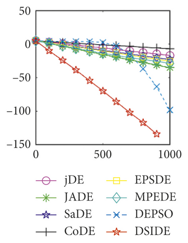
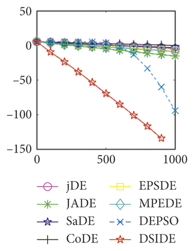
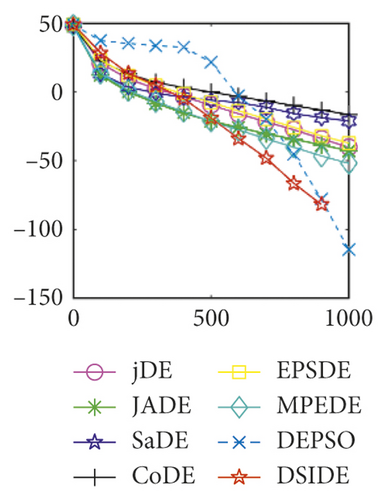
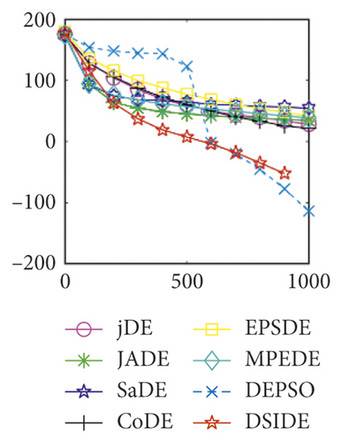
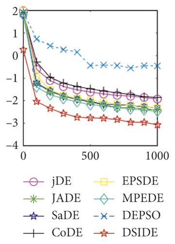
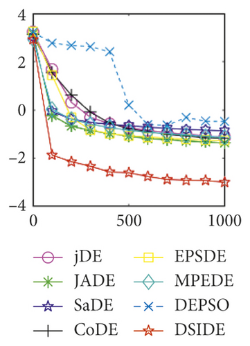
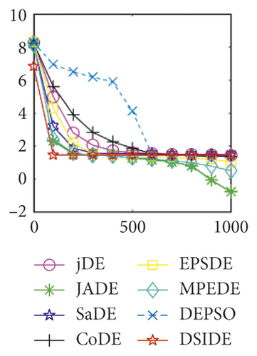
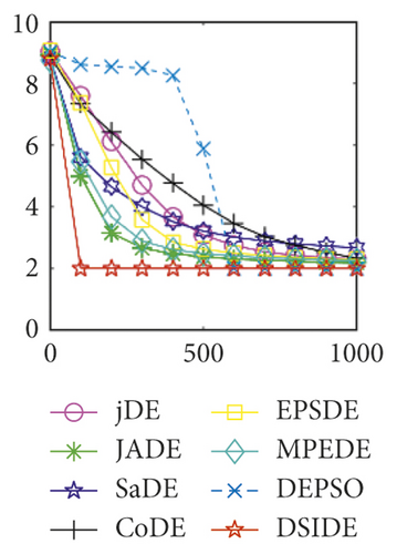
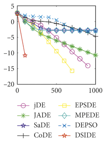
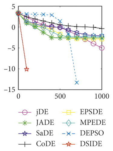
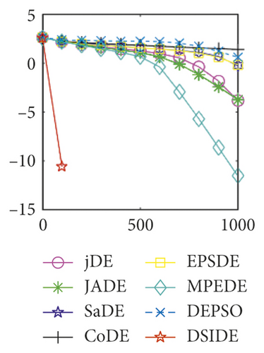
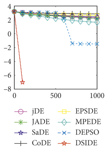
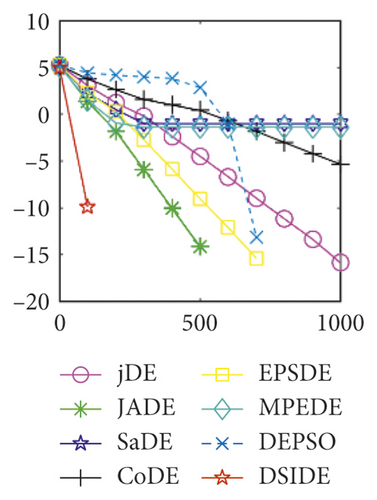
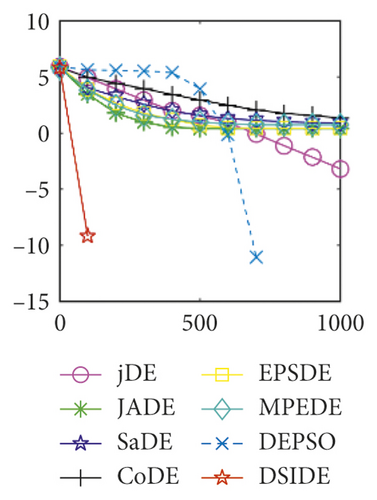
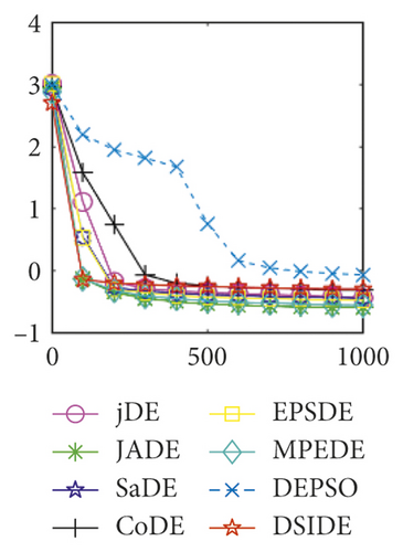
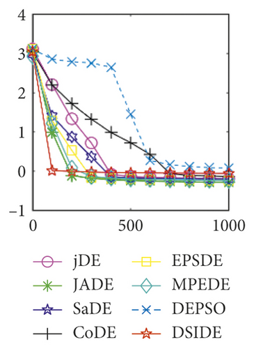
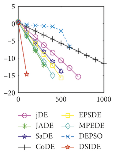
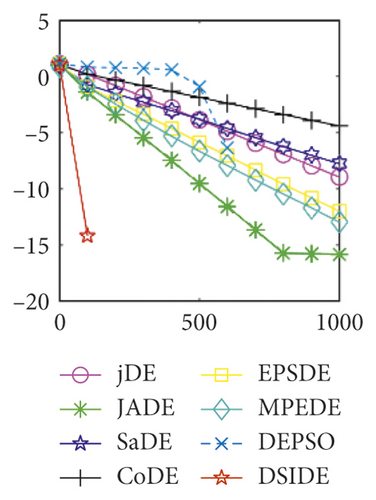
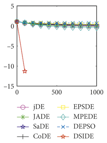
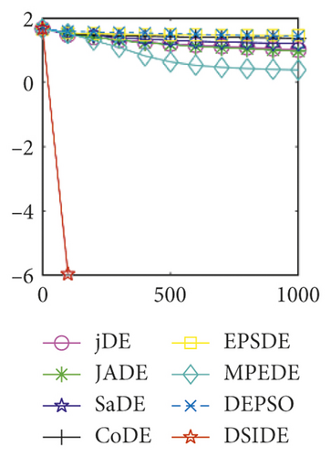
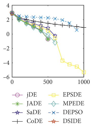
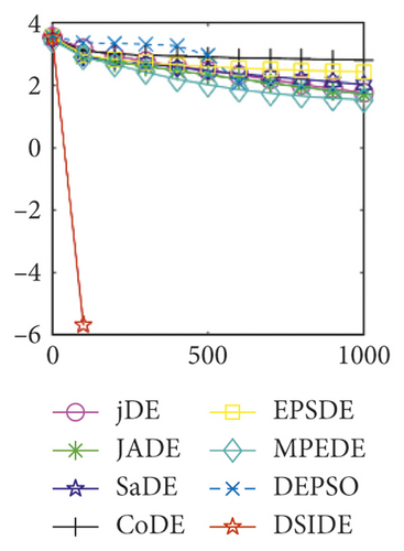
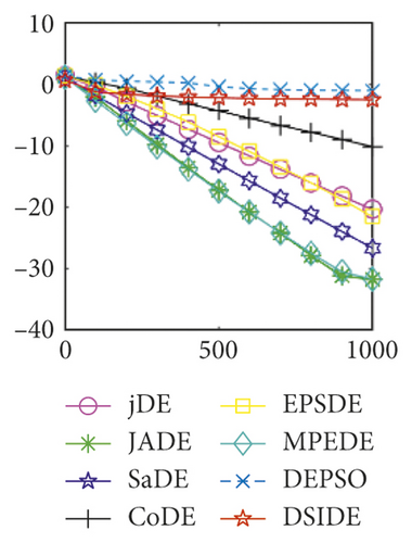
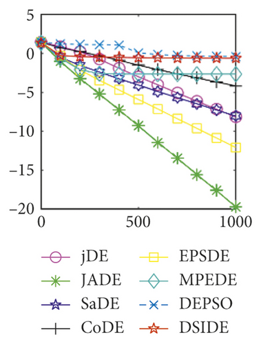
Furthermore, we compare the convergence curves of each algorithm on benchmark functions at 30 D and 100 D. All convergence curves are studied and analyzed from the aspects of convergence precision and whether they converge to the global optimum or not. Some representative convergence curves are depicted in Figures 1 and 2.

As shown in Figures 1(a) and 1(b), in convergence curves of function f₁ at 30 D and 100 D, only DSIDE converges to the global optimum, and the average convergence accuracy is much higher than other algorithms under the same generations. Convergence curves of f₇, as shown in Figures 1(c)and 1(d). Although convergence precision is not always optimal in the evolution process, only DSIDE gets the global optimum. Figures 1(e) and 1(f) show convergence curves of f₁₃ at 30 D and 100 D, respectively. All algorithms have not found the optimal solution, but the average convergence accuracy of DSIDE is much higher than other algorithms under the same generations and obtains the best value. Figures 1(g) and 1(h) show convergence curves of f₁₄ at 30 D and 100 D, respectively. All algorithms have not obtained the global minimum. JADE performs the best on the low-dimensional problem, while DSIDE is the best on high-dimensional. In Figures 1(i) and 1(j), DSIDE converges the fastest on f₁₅. DSIDE, EPSDE, and jDE converge to the global optimum at 30 D, while DSIDE and DEPSO reach the optimal at 100 D. In Figures 1(k) and 1(l), only DSIDE gets the global optimal on f₁₆ and consumes fewer generations and converges quickly.

In Figure 2(a), DSIDE, JADE, DEPSO, and EPSDE obtain the optimal on f₁₈ at 30 D. In Figure 2(b), DSIDE and DEPSO get the global optimal on f₁₈ at 100D. DSIDE has the fastest convergence speed in both low-dimensional and high-dimensional problems. Convergence curves of function f₂₃ in Figures 2(c) and 2(d), none of the algorithms finds the global minimum, and there is a phenomenon of “evolutionary stagnation.” In Figures 2(e) and 2(f) on function f₂₅, only CoDE cannot find the global minimum at 30D; DSIDE and DEPSO get the global optimal at 100D, but the former costs much less generations. In Figures 2(g) and 2(h), DSIDE converges to the global optimal on f₂₆, while other algorithms suffer from “evolutionary stagnation.” In Figure 2(i), the global minimum value is found by all algorithms except CoDE and EPSDE on f₂₈ at 30 D. In Figure 2(j), DSIDE and DEPSO get the global optimal on function f₂₈ at 100 D. In Figures 2(k) and 2(l), DSIDE performs relatively low but consistently outperforms DEPSO on function f₂₉.

In general, through the comparative analysis of the above experiments, DSIDE not only obtains the global optimal value most times on these benchmark functions but also is superior to other algorithms in terms of convergence speed and convergence accuracy.

4.3. Efficiency Analysis of Proposed Algorithmic Components

So far, the above experiment exhibits the combined effect of the proposed DSIDE. In this section, the efficiency analysis of proposed algorithmic components is completed, including the enhanced mutation strategy of the reference factor and the adaptive strategy of the scaling factor and crossover probability. Some variants of DSIDE are listed as follows:

(i
)To verify the effectiveness of the enhanced mutation strategy of reference factor α, DSIDE variants adopt dynamic F, CR, and constant reference factor of α = 0.3 and α = 0.6 and random real number in [0,1], which are, respectively, called as DSIDE-1, DSIDE-2, and DSIDE-3 one by one.
(ii)
To investigate the validity of the scaling factor adaptive strategy, DSIDE variants employ dynamic CR, α and fixed scaling factor of F = 0.3, F = 0.6, and random real number in [0,1], which are named DSIDE -4, DSIDE -5, and DSIDE -6 for short.
(iii)
To study the contribution of the crossover probability adaptive strategy, DSIDE variants with shifty F, α and settled crossover probability of CR = 0.3 and CR = 0.6, and random real number in [0,1] are, respectively, abbreviated as DSIDE-7, DSIDE-8, and DSIDE-9.

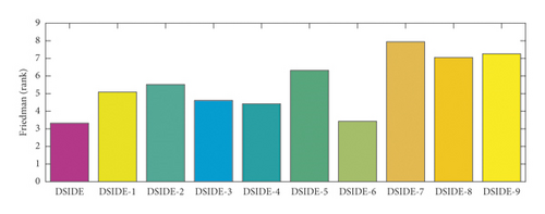
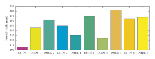
For the purpose of evaluating and comparing the performance of DSIDE variants, Friedman test, Kruskal–Wallis test, and Wilcoxon’s rank-sum test are adopted, and the test results are shown in Figure 3(a), Figure 3(b), and Table 7, respectively. The following summaries can be obtained. (1) From Figure 3, we can observe that DSIDE and DSIDE-6 are the best and the second, while the performance of other DSIDE variants is relatively low. The combined effect of the proposed algorithmic components is the best. (2) From Table 7, the integrated DSIDE performs significantly better than DSIDE variants (DSIDE-2 and DSIDE-5) with a larger reference factor and a lager scaling factor, as well as DSIDE variants (DSIDE-7, DSIDE-8, and DSIDE-9) with different crossover probability. The performance between the integrated DSIDE and DSIDE-1 with a smaller reference factor, DSIDE-3 with a random reference factor, and DSIDE-4 with a smaller scaling factor show no significant difference when the significance level of Wilcoxon’s rank-sum test is 0.1, but the difference is opposite when the significant level is 0.05. At the same time, there is no performance difference between DSIDE and DSIDE-6 with a random scaling factor, regardless of the significance level. The validity of the proposed mutation strategy and adaptive strategy for control parameters is demonstrated utilizing above experimental comparisons. It is noted that the contribution of the adaptive strategy of crossover probability is larger than enhanced mutation strategy and adaptive strategy of scaling factor. That is to say, although the enhanced mutation strategy of reference factor and adaptive strategy of scaling factor are effective, DSIDE is less susceptible to both a smaller or variational reference factor and scaling factor.

Table 7. Wilcoxon’s rank-sum test results of proposed DSIDE and 9 DSIDE variants over 30 independent runs.

Comparison	D = 30
Comparison	R⁺	R⁻	p value	α = 0.05	α = 0.1
DSIDE vs. DSIDE-1	216	37	1.12e − 02	No	Yes
DSIDE vs. DSIDE-2	165	135	5.63e − 03	Yes	Yes
DSIDE vs. DSIDE-3	154	122	1.34e − 02	No	Yes
DSIDE vs. DSIDE-4	75	30	2.21e − 01	No	No
DSIDE vs. DSIDE-5	194	106	5.63e − 03	Yes	Yes
DSIDE vs. DSIDE-6	59	46	3.00e − 01	No	No
DSIDE vs. DSIDE-7	242	34	2.94e − 03	Yes	Yes
DSIDE vs DSIDE-8	276	0	6.46e − 03	Yes	Yes
DSIDE vs DSIDE-9	276	0	7.45e − 03	Yes	Yes

5. Conclusions

DSIDE’s innovation lies in two strategies, the enhanced mutation strategy and the novel adaptive strategy for control parameters. On the one hand, the enhanced mutation strategy considers the influence of the reference individual on the overall evolution. It introduces the reference factor, which is beneficial to global exploration in the early stage of evolution and global convergence in the later stage. On the other hand, the novel adaptive strategy for control parameters can dynamically adjust the scaling factor and crossover probability according to the fitness value, which has a positive impact on maintaining the population diversity. DSIDE is compared with other seven DE algorithms, the results are evaluated by three nonparametric statistical tests, and the convergence curves are analyzed. Experimental results show that the proposed DSIDE can effectively improve the optimization performance. Besides, the efficiency analysis of proposed algorithmic components has been carried out, which further proves the comprehensive effect and validity of DSIDE.

So far, DE variants have been applied to various fields, such as target allocation [41], text classification [42], image segmentation [43], and neural network [44–47]. For the future work, the proposed DSIDE algorithm will be applied to the parameter optimization of neural network and may further apply it to the air traffic control system for flight trajectory prediction [48, 49].

Conflicts of Interest

The authors declare that there are no conflicts of interest regarding the publication of this paper.

Acknowledgments

This work was supported by the National Natural Science Foundation of China, no. U1833128.

Open Research

Data Availability

The data used to support the findings of this study are available from the corresponding author upon request.

References

1 Storn R. and Price K., Differential evolution: a simple and efficient adaptive scheme for global optimization over continuous spaces, Journal of Global Optimization. (1995) 23, no. 1.
Google Scholar
2 Eiben A. E., Hinterding R., and Michalewicz Z., Parameter control in evolutionary algorithms, IEEE Transactions on Evolutionary Computation. (1999) 3, no. 2, 124–141, https://doi.org/10.1109/4235.771166, 2-s2.0-0032626111.
10.1109/4235.771166
Web of Science® Google Scholar
3 Karafotias G., Hoogendoorn M., and Eiben A. E., Parameter control in evolutionary algorithms: trends and challenges, IEEE Transactions on Evolutionary Computation. (2015) 19, no. 2, 167–187, https://doi.org/10.1109/tevc.2014.2308294, 2-s2.0-84926472380.
10.1109/TEVC.2014.2308294
Web of Science® Google Scholar
4 Omran M. G. H., Salman A., and Engelbrecht A. P., Self-adaptive differential evolution, Proceedings of the International Conference on Computational Intelligence and Security, 2005, Xi’an, China.
Google Scholar
5 Liu J. and Lampinen J., A fuzzy adaptive differential evolution algorithm, Soft Computing. (2005) 9, no. 6, 448–462, https://doi.org/10.1007/s00500-004-0363-x, 2-s2.0-20444409462.
10.1007/s00500-004-0363-x
Web of Science® Google Scholar
6 Brest J., Greiner S., Boskovic B., Mernik M., and Zumer V., Self-adapting control parameters in differential evolution: a comparative study on numerical benchmark problems, IEEE Transactions on Evolutionary Computation. (2006) 10, no. 6, 646–657, https://doi.org/10.1109/tevc.2006.872133, 2-s2.0-33847199831.
10.1109/TEVC.2006.872133
Web of Science® Google Scholar
7 Noman N., Bollegala D., and Iba H., An adaptive differential evolution algorithm, Proceedings of the IEEE Congress of Evolutionary Computation, 2011, New Orleans, LA, USA, IEEE.
Google Scholar
8 Asafuddoula M., Ray T., and Sarker R., An adaptive hybrid differential evolution algorithm for single objective optimization, Applied Mathematics and Computation. (2014) 231, 601–618, https://doi.org/10.1016/j.amc.2014.01.041, 2-s2.0-84893299538.
10.1016/j.amc.2014.01.041
Web of Science® Google Scholar
9 Tanabe R. and Fukunaga A., Success-history based parameter adaptation for differential evolution, Proceedings of the 2013 IEEE Congress on Evolutionary Computation, June 2013, Cancun, Mexico, IEEE, 71–78, https://doi.org/10.1109/CEC.2013.6557555, 2-s2.0-84881600175.
10.1109/CEC.2013.6557555
Google Scholar
10 Tanabe R. and Fukunaga A. S., Improving the search performance of shade using linear population size reduction, Proceedings of the 2014 IEEE Congress on Evolutionary Computation, 2014, Beijing, China, IEEE, 1658–1665, https://doi.org/10.1109/CEC.2014.6900380, 2-s2.0-84908582441.
10.1109/CEC.2014.6900380
Google Scholar
11 Zhu W., Tang Y., Fang J.-A., and Zhang W., Adaptive population tuning scheme for differential evolution, Information Sciences. (2013) 223, 164–191, https://doi.org/10.1016/j.ins.2012.09.019, 2-s2.0-84870241188.
10.1016/j.ins.2012.09.019
Web of Science® Google Scholar
12 Zhao S., Wang X., Chen L., and Zhu W., A novel self-adaptive differential evolution algorithm with population size adjustment scheme, Arabian Journal for Science and Engineering. (2014) 39, no. 8, 6149–6174, https://doi.org/10.1007/s13369-014-1248-7, 2-s2.0-84904894114.
10.1007/s13369-014-1248-7
Google Scholar
13 Pan J. S., Yang C., Meng F. J., Chen Y. X., and Meng Z. Y., A parameter adaptive DE algorithm on real-parameter optimization, Journal of Intelligent and Fuzzy Systems. (2020) 38, no. 1, 1–12, https://doi.org/10.3233/jifs-179665.
10.3233/JIFS-179665
Google Scholar
14 Meng Z., Chen Y., and Li X., Enhancing differential evolution with novel parameter control, IEEE Access. (2020) 8, 51145–51167, https://doi.org/10.1109/access.2020.2979738.
10.1109/ACCESS.2020.2979738
Google Scholar
15 Di Carlo M., Vasile M., and Minisci E., Adaptive multi-population inflationary differential evolution, Soft Computing. (2020) 24, no. 5, 3861–3891, https://doi.org/10.1007/s00500-019-04154-5, 2-s2.0-85068973808.
10.1007/s00500-019-04154-5
Google Scholar
16 Wales D. and Doye J., Global optimization by basin-hopping and the lowest energy structures of lennard-jones clusters containing up to 110 atoms, Journal of Physical Chemistry A. (1998) 101, no. 28, 5111–5116.
10.1021/jp970984n
Google Scholar
17 Li S., Gu Q., Gong W., and Ning B., An enhanced adaptive differential evolution algorithm for parameter extraction of photovoltaic models, Energy Conversion and Management. (2020) 205, 112443, https://doi.org/10.1016/j.enconman.2019.112443.
10.1016/j.enconman.2019.112443
Web of Science® Google Scholar
18 Das S., Abraham A., Chakraborty U. K., and Konar A., Differential evolution using a neighborhood-based mutation operator, IEEE Transactions on Evolutionary Computation. (2009) 13, no. 3, 526–553, https://doi.org/10.1109/tevc.2008.2009457, 2-s2.0-65749094710.
10.1109/TEVC.2008.2009457
Web of Science® Google Scholar
19 Zhang J. Q. and Sanderson A. C., JADE: adaptive differential evolution with optional external archive, IEEE Transactions on Evolutionary Computation. (2009) 13, no. 5, 945–958.
10.1109/TEVC.2009.2014613
Web of Science® Google Scholar
20 Qin A. K., Huang V. L., and Suganthan P. N., Differential evolution algorithm with strategy adaptation for global numerical optimization, IEEE Transactions on Evolutionary Computation. (2009) 13, no. 2, 398–417, https://doi.org/10.1109/tevc.2008.927706, 2-s2.0-59649083826.
10.1109/TEVC.2008.927706
Web of Science® Google Scholar
21 Wang Y., Cai Z., and Zhang Q., Differential evolution with composite trial vector generation strategies and control parameters, IEEE Transactions on Evolutionary Computation. (2011) 15, no. 1, 55–66, https://doi.org/10.1109/tevc.2010.2087271, 2-s2.0-79952003746.
10.1109/TEVC.2010.2087271
CAS Web of Science® Google Scholar
22 Epitropakis M. G., Tasoulis D. K., Pavlidis N. G., Plagianakos V. P., and Vrahatis M. N., Enhancing differential evolution utilizing proximity-based mutation operators, IEEE Transactions on Evolutionary Computation. (2011) 15, no. 1, 99–119, https://doi.org/10.1109/tevc.2010.2083670, 2-s2.0-79952004145.
10.1109/TEVC.2010.2083670
Web of Science® Google Scholar
23 Mallipeddi R., Suganthan P. N., Pan Q. K., and Tasgetiren M. F., Differential evolution algorithm with ensemble of parameters and mutation strategies, Applied Soft Computing. (2011) 11, no. 2, 1679–1696, https://doi.org/10.1016/j.asoc.2010.04.024, 2-s2.0-78650872465.
10.1016/j.asoc.2010.04.024
Web of Science® Google Scholar
24 Xiang W. L., Meng X. L., An M. Q., Li Y. Z., and Gao M. X., An enhanced differential evolution algorithm based on multiple mutation strategies, Computational Intelligence and Neuroscience. (2015) 2015, 15, 285730, https://doi.org/10.1155/2015/285730, 2-s2.0-84947557249.
10.1155/2015/285730
PubMed Google Scholar
25 Cui L., Li G., Lin Q., Chen J., and Lu N., Adaptive differential evolution algorithm with novel mutation strategies in multiple sub-populations, Computers & Operations Research. (2016) 67, 155–173, https://doi.org/10.1016/j.cor.2015.09.006, 2-s2.0-84946599641.
10.1016/j.cor.2015.09.006
Web of Science® Google Scholar
26 Wu G., Mallipeddi R., Suganthan P. N., Wang R., and Chen H., Differential evolution with multi-population based ensemble of mutation strategies, Information Sciences. (2016) 329, 329–345, https://doi.org/10.1016/j.ins.2015.09.009, 2-s2.0-84949651247.
10.1016/j.ins.2015.09.009
Web of Science® Google Scholar
27 Meng Z., Pan J.-S., and Kong L., Parameters with adaptive learning mechanism (palm) for the enhancement of differential evolution, Knowledge-Based Systems. (2018) 141, 92–112, https://doi.org/10.1016/j.knosys.2017.11.015, 2-s2.0-85034455273.
10.1016/j.knosys.2017.11.015
Web of Science® Google Scholar
28 Meng Z., Pan J.-S., and Tseng K.-K., PaDE: an enhanced differential evolution algorithm with novel control parameter adaptation schemes for numerical optimization, Knowledge-Based Systems. (2019) 168, 80–99, https://doi.org/10.1016/j.knosys.2019.01.006, 2-s2.0-85059863343.
10.1016/j.knosys.2019.01.006
Web of Science® Google Scholar
29 Wei Z., Xie X., Bao T., and Yu Y., A random perturbation modified differential evolution algorithm for unconstrained optimization problems, Soft Computing. (2019) 23, no. 15, 6307–6321, https://doi.org/10.1007/s00500-018-3285-8, 2-s2.0-85048365383.
10.1007/s00500-018-3285-8
Google Scholar
30 Duan M., Yang H., Liu H., and Chen J., A differential evolution algorithm with dual preferred learning mutation, Applied Intelligence. (2019) 49, no. 2, 605–627, https://doi.org/10.1007/s10489-018-1267-2, 2-s2.0-85053452652.
10.1007/s10489-018-1267-2
Google Scholar
31 Tian M. and Gao X., Differential evolution with neighborhood-based adaptive evolution mechanism for numerical optimization, Information Sciences. (2019) 478, 422–448, https://doi.org/10.1016/j.ins.2018.11.021, 2-s2.0-85056848655.
10.1016/j.ins.2018.11.021
Web of Science® Google Scholar
32 Wang S. H., Li Y. Z., and Yang H. Y., Self-adaptive mutation differential evolution algorithm based on particle swarm optimization, Applied Soft Computing. (2019) 81.
10.1016/j.asoc.2019.105496
Google Scholar
33 Meng Z. and Pan J.-S., HARD-DE: hierarchical archive based mutation strategy with depth information of evolution for the enhancement of differential evolution on numerical optimization, IEEE Access. (2019) 7, 12832–12854, https://doi.org/10.1109/access.2019.2893292, 2-s2.0-85061308769.
10.1109/ACCESS.2019.2893292
Google Scholar
34 Zheng L. M., Zhang S. X., Tang K. S., and Zheng S. Y., Differential evolution powered by collective information, Information Sciences. (2017) 399, 13–29, https://doi.org/10.1016/j.ins.2017.02.055, 2-s2.0-85014845427.
10.1016/j.ins.2017.02.055
Web of Science® Google Scholar
35 Pan J.-S., Liu N., and Chu S.-C., A hybrid differential evolution algorithm and its application in unmanned combat aerial vehicle path planning, IEEE Access. (2020) 8, 17691–17712, https://doi.org/10.1109/access.2020.2968119.
10.1109/ACCESS.2020.2968119
Web of Science® Google Scholar
36 Meng Z., Yang C., Li X., and Chen Y., Di-DE: depth information-based differential evolution with adaptive parameter control for numerical optimization, IEEE Access. (2020) 8, 40809–40827, https://doi.org/10.1109/access.2020.2976845.
10.1109/ACCESS.2020.2976845
Web of Science® Google Scholar
37 Liang J. J., Qu B. Y., Suganthan P. N., and Chen Q., Problem definition and evaluation criteria for the cec 2015 competition on learning based real-parameter single objective optimization, 2015.
Google Scholar
38 Awad N. H., Ali M. Z., Suganthan P. N., Liang J. J., and Qu B. Y., Problem definitions and evaluation criteria for the CEC 2017 special session and competition on single objective real-Parameter numerical optimization, 2016.
Google Scholar
39 Bilal P. M., Pant M., Zaheer H., Garcia-Hernandez L., and Abraham A., Differential evolution: a review of more than two decades of research, Engineering Applications of Artificial Intelligence. (2020) 90, https://doi.org/10.1016/j.engappai.2020.103479.
10.1016/j.engappai.2020.103479
Google Scholar
40 Derrac J., García S., Molina D., and Herrera F., A practical tutorial on the use of nonparametric statistical tests as a methodology for comparing evolutionary and swarm intelligence algorithms, Swarm and Evolutionary Computation. (2011) 1, no. 1, 3–18, https://doi.org/10.1016/j.swevo.2011.02.002, 2-s2.0-79960535211.
10.1016/j.swevo.2011.02.002
Web of Science® Google Scholar
41 Bayrak A. E. and Polat F., Employment of an evolutionary heuristic to solve the target allocation problem efficiently, Information Sciences. (2013) 222, no. 3, 675–695, https://doi.org/10.1016/j.ins.2012.07.050, 2-s2.0-84870058738.
10.1016/j.ins.2012.07.050
Web of Science® Google Scholar
42 Onan A., Korukoğlu S., and Bulut H., A multiobjective weighted voting ensemble classifier based on differential evolution algorithm for text sentiment classification, Expert Systems with Applications. (2016) 62, 1–16, https://doi.org/10.1016/j.eswa.2016.06.005, 2-s2.0-84977070618.
10.1016/j.eswa.2016.06.005
Web of Science® Google Scholar
43 Tarkhaneh O. and Shen H. F., An adaptive differential evolution algorithm to optimal multi-level thresholding for MRI brain image segmentation, Expert Systems with Applications. (2019) 138.
10.1016/j.eswa.2019.07.037
Google Scholar
44 Subudhi B. and Jena D., A differential evolution based neural network approach to nonlinear system identification, Applied Soft Computing. (2011) 11, no. 1, 861–871, https://doi.org/10.1016/j.asoc.2010.01.006, 2-s2.0-77957914596.
10.1016/j.asoc.2010.01.006
Web of Science® Google Scholar
45 Dhahri H., Alimi A. M., and Abraham A., Hierarchical multi-dimensional differential evolution for the design of beta basis function neural network, Neurocomputing. (2012) 97, 131–140, https://doi.org/10.1016/j.neucom.2012.04.008, 2-s2.0-84865324245.
10.1016/j.neucom.2012.04.008
Google Scholar
46 Lu H.-C., Chang M.-H., and Tsai C.-H., Parameter estimation of fuzzy neural network controller based on a modified differential evolution, Neurocomputing. (2012) 89, 178–192, https://doi.org/10.1016/j.neucom.2012.02.017, 2-s2.0-84860234660.
10.1016/j.neucom.2012.02.017
Web of Science® Google Scholar
47 Piotrowski A. P., Differential Evolution algorithms applied to neural network training suffer from stagnation, Applied Soft Computing. (2014) 21, 382–406, https://doi.org/10.1016/j.asoc.2014.03.039, 2-s2.0-84899525106.
10.1016/j.asoc.2014.03.039
Web of Science® Google Scholar
48 Hong S. and Lee K., Trajectory prediction for vectored area navigation arrivals, Journal of Aerospace Information Systems. (2015) 12, no. 7, 490–502, https://doi.org/10.2514/1.i010245, 2-s2.0-84940773159.
10.2514/1.I010245
Web of Science® Google Scholar
49 Gallego C. E. V., Gomez V. F., Carmona M. A. A., Valdes R. M. A., Nieto F. J. S., and Martinez M. G., A machine learning approach to air traffic interdependency modelling and its application to trajectory prediction, Transportation Research Part C: Emerging Technologies. (2019) 107, 356–386.
10.1016/j.trc.2019.08.015
Google Scholar

Citing Literature

All articles

An Improved Differential Evolution Algorithm Based on Dual-Strategy

Abstract

1. Introduction