Volume 2020, Issue 1 6468909

Research Article

Open Access

Estimating Rice Panicle Temperature with Three-Layer Model

Yanyan Wang

Jiangxi Agricultural University, 1101 Zhimin Road, Economic and Technological Development Zone, Nanchang, 330045 Jiangxi, China jxau.edu.cn

Search for more papers by this author

Hiroki Oue,

Corresponding Author

Hiroki Oue

[email protected]

orcid.org/0000-0001-5806-0952

Faculty of Agriculture, Ehime University, 3-5-7 Tarumi, Matsuyama, Ehime 7908566, Japan ehime-u.ac.jp

Search for more papers by this author

Zhijun Luo,

Corresponding Author

Zhijun Luo

[email protected]

orcid.org/0000-0003-4205-7155

Jiangxi Agricultural University, 1101 Zhimin Road, Economic and Technological Development Zone, Nanchang, 330045 Jiangxi, China jxau.edu.cn

Search for more papers by this author

Ming Chen,

Ming Chen

Hunan University, Lushan Road (S) Yuelu District, Changsha, Hunan 410082, China hnu.edu.cn

Search for more papers by this author

Shiyu Liu,

Shiyu Liu

Jiangxi Agricultural University, 1101 Zhimin Road, Economic and Technological Development Zone, Nanchang, 330045 Jiangxi, China jxau.edu.cn

Search for more papers by this author

Chunhuo Zhou,

Chunhuo Zhou

Jiangxi Agricultural University, 1101 Zhimin Road, Economic and Technological Development Zone, Nanchang, 330045 Jiangxi, China jxau.edu.cn

Search for more papers by this author

Xiaowu He,

Xiaowu He

Jiangxi Agricultural University, 1101 Zhimin Road, Economic and Technological Development Zone, Nanchang, 330045 Jiangxi, China jxau.edu.cn

Search for more papers by this author

Yanyan Wang,

Yanyan Wang

Jiangxi Agricultural University, 1101 Zhimin Road, Economic and Technological Development Zone, Nanchang, 330045 Jiangxi, China jxau.edu.cn

Search for more papers by this author

Hiroki Oue,

Corresponding Author

Hiroki Oue

[email protected]

orcid.org/0000-0001-5806-0952

Faculty of Agriculture, Ehime University, 3-5-7 Tarumi, Matsuyama, Ehime 7908566, Japan ehime-u.ac.jp

Search for more papers by this author

Zhijun Luo,

Corresponding Author

Zhijun Luo

[email protected]

orcid.org/0000-0003-4205-7155

Jiangxi Agricultural University, 1101 Zhimin Road, Economic and Technological Development Zone, Nanchang, 330045 Jiangxi, China jxau.edu.cn

Search for more papers by this author

Ming Chen,

Ming Chen

Hunan University, Lushan Road (S) Yuelu District, Changsha, Hunan 410082, China hnu.edu.cn

Search for more papers by this author

Shiyu Liu,

Shiyu Liu

Jiangxi Agricultural University, 1101 Zhimin Road, Economic and Technological Development Zone, Nanchang, 330045 Jiangxi, China jxau.edu.cn

Search for more papers by this author

Chunhuo Zhou,

Chunhuo Zhou

Jiangxi Agricultural University, 1101 Zhimin Road, Economic and Technological Development Zone, Nanchang, 330045 Jiangxi, China jxau.edu.cn

Search for more papers by this author

Xiaowu He,

Xiaowu He

Jiangxi Agricultural University, 1101 Zhimin Road, Economic and Technological Development Zone, Nanchang, 330045 Jiangxi, China jxau.edu.cn

Search for more papers by this author

First published: 20 March 2020

https://doi.org/10.1155/2020/6468909

Citations: 1

Academic Editor: Hiroyuki Hashiguchi

Share a link

Email
Wechat
Bluesky

Abstract

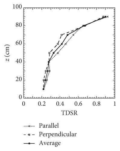
Rice panicle temperature (T_p) is a key factor for studying high temperature impacts on spikelet sterility. Comparing with measuring T_p by hand, a T_p simulation model could obtain T_p data readily. The two-layer energy budget model which divides the soil layer and canopy layer was widely used to predict rice canopy temperature (T_c), but panicle existed mostly in the upper layer canopy, and we have proved that T_c was different from the upper layer canopy temperature (T_c1), and the upper layer must be separated from the whole canopy for the purpose of estimating T_p. Thus, we developed the three-layer model, contained upper canopy layer with panicle (50–100 cm), lower rice canopy layer (10–40 cm), and water surface layer (≤10 cm) to estimate T_p with general meteorological and vegetation growth data. There were two steps to estimate T_p. The first step was calculating T_c1 and lower layer canopy temperature (T_c2) by solving heat balance equations with canopy resistances. And the second step was estimating T_p with following parameters: (a) the inclination factors of leaves and panicles (F₁, F₂, and F_p) which were decided by fitting the calculated transmissivity of downward solar radiation (TDSR) to the measured TDSR, (b) the aerodynamic resistance between the panicle and atmosphere (r_ap) denoted by wind speed, (c) the panicle resistance for transpiration (r_p) denoted by days after heading, and (d) air temperature and humidity at the panicle’s height (T_ac1 and e_ac1) calculated from the resistances of the pathways of sensible and latent heat fluxes in accordance with Ohm’s law. The model simulated fairly well the T_c1, T_c2, and T_p with root mean square errors (RMSEs) of 0.76°C, 0.75°C, and 0.81°C, respectively, where RMSE of measured T_p and predicted T_p by integrated micrometeorology model for panicle and canopy temperature (IM²PACT) including two-layer model was 1.27°C. This model was validated well by two other rice cultivars, and thus, it demonstrated the three-layer model was a new feasible way to estimate T_p.

1. Introduction

With increasing concerns about global warming, the impacts of higher temperature on rice production have become a major focus in many rice-producing countries in tropical, subtropical, and temperate regions [1–9]. In China, extreme high temperature in 2003 caused about 5 million tonnes of rice yield loss [10], while unusual temperatures (>40°C) in many areas of Kanto and Tokai regions of Japan resulted in 25% spikelet sterility in 2007 [11].

Rice panicle is most sensitive to high temperature during the flowering stage [12–16]. It has been proved that high temperature prevents anther dehiscence and decreases basal pore length of the anther, resulting in low numbers of germinating pollen grains on the stigma, and thus, it causes spikelet sterility [7, 12, 15, 17–22].

Effect of high temperature on spikelet sterility has been studied under different conditions. Matsui et al. [23] reported that spikelet fertility was significantly damaged when daily maximum air temperature exceeded 35°C. Abeysiriwardena et al. [24] revealed high temperature condition (35°C day/30°C night) induced complete grain sterility when relative humidity (RH) was 85–95%. Contrary to the results above, [25, 26] demonstrated spikelet sterility of rice did not occur seriously even daily maximum T_a was over 40°C in Australia during the 2004–2006 growing seasons because the strong transpirational cooling by low relative humidity (<20%) brought panicle temperature (T_p) 6.8°C lower than T_a. But spikelet sterility occurred frequently in Jianghan Basin, China, where T_a was not so high, since T_p was 4.0°C higher than T_a under high solar radiation with high RH (>80%) and low wind speed (u < 1 m s⁻¹) conditions [27]. Therefore, T_p instead of T_a is a key factor for high temperature impact study. As measuring T_p was a time-consuming and laborious work, a T_p simulation model was needed to obtain T_p data readily.

Until now, only limited information has been reported about panicle temperature models. Sheehy et al. [28] developed a T_p model with air temperature and thermal burden. Oue et al. [29] measured T_p in every 10 cm rice canopy layer in the CO₂ ambient and CO₂ elevated plots during the daytime in Wuxi, China, and developed a heat balance model of T_p based on the measured stomatal conductance. To date, the whole canopy temperature (T_c) predicted by the two-layer model has been used to calculate the long-wave radiations to the panicle as shown in the integrated micrometeorology model for panicle and canopy temperature (IM²PACT) [30]. However, panicle exists mostly in the upper layer canopy, and we have proved that T_c is different from the upper layer canopy temperature (T_c1), and the upper layer must be separated from the whole canopy for the purpose of estimating T_p, whereas the multilayer model [31] required many vertical profiles of micrometeorological environments and fluxes of momentum, and heat and vapor within and above a vegetation, making it unusable to predict T_p with insufficient data.

Therefore, the objectives of this paper are (1) to develop a three-layer model to calculate panicle temperature based on general meteorological and vegetation growth data and (2) to compare the performance to estimate T_p by three-layer model and T_p by IM²PACT [30] including two-layer model.

2. Materials and Methods

2.1. Measurements in the Rice Paddy Field

The experimental paddy field was located in the Ehime University Senior High School, Matsuyama, Japan (33°50′N, 132°47′E). The Japonica type rice (cultivar Akitakomachi) was transplanted with 20 × 30 cm spacing on May 27, 2014, and then harvested on September 8, 2014.

The global solar radiation (S_t), downward long-wave radiation (L_d), and upward long-wave radiation (L_u) above the rice canopy were detected using pyranometer CNR-4 (Kipp & Zonen, the Netherlands) at 2.0 m height from the ground. To measure soil heat flux (G), a soil heat plate CHF-HDP01 (Campbell Scientific Inc., Logan, UT, USA) was buried in the soil surface. Air temperature (T_a) and relative humidity (RH) were observed using ventilated psychrometers HMP-45A (Vaisala Inc., Helsinki, Finland), first mounted at 0.6 m and 1.0 m of a 2.5 m tower, and then lifted to 1.0 m and 1.5 m on July 28, respectively, when rice plant was 81 cm in height. Three-cup anemometers 014A (MetOne, USA) were mounted as the same heights of psychrometers to measure the wind speed (u). Downward and upward long-wave radiations beneath the rice canopy were both measured with PRI-01 (Prede, Japan) sensors. Water surface temperature (T_w) or ground surface temperature (T_g) was measured with the thermocouple sensor. All data were sampled per 10 s; then, they were averaged and recorded per 10 min using a data logger CR23x (Campbell Scientific Inc., Logan, UT, USA).

Three stubs of rice were taken to measure the upper layer canopy temperature (T_c1), the lower layer canopy temperature (T_c2), and the panicle temperature (T_p) per 2 or 3 h in the daytime using an infrared thermometer THI-500 (Tasco, Japan). The solar radiation within rice canopy was measured with a line type pyranometer PCM200 (Prede, Japan) in the center between stubs in parallel and perpendicular directions, of which the average was calibrated from the solar radiation measured with CNR-4 (Kipp & Zonen, the Netherlands) at 2.0 m. The transmissivity of downward solar radiation (TDSR) refers to the ratio of the St in the rice canopy in every 10 cm to that above the rice canopy. Subsequently, the average TDSRs from 50 cm to 100 cm and from 10 cm to 40 cm were set as the upper and lower layer rice canopy TDSRs, respectively. TDSRs were measured from 10 cm to the top of the canopy per 10 cm and 1.2 m (above the rice canopy). The canopy temperature, T_p, and solar radiation within canopy data were recorded using ZR-RX 20 portable multilogger (Omron, Japan). At the heading and the flowering stage, irrigation was performed in the paddy field at 5-day interval. Besides, 8 cm depth irrigation water decreased to 0 through evaporation and infiltration in one and a half days. At the ripening stage, there was almost no water.

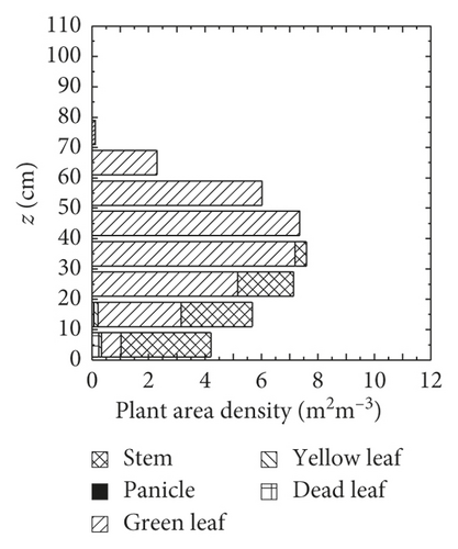
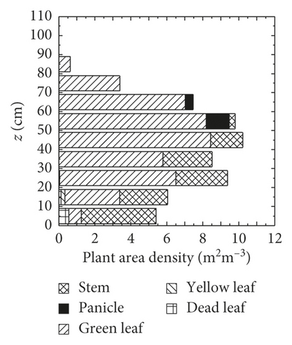
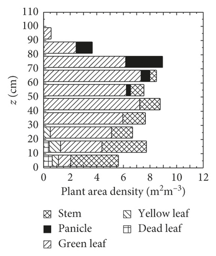
Plant area density (PAD) was sampled three rice plants at the interval of one week. The taken three rice plants were cut at intervals of 10 cm, split into components of leaves, stems, and panicles, respectively, and then scanned. Lastly, the area of each part (projected area for panicle) was calculated using ImageJ software. Water depth (d_w) was measured per two or three hours in the daytime. Water surface evaporation (E_g) beneath the rice canopy was measured with the lysimeter (length × width × depth: 60 × 20 × 30 cm) and recorded twice (8:30 and 18:30) per day.

2.2. Estimating Panicle Temperature (T_p) with Three-Layer Model

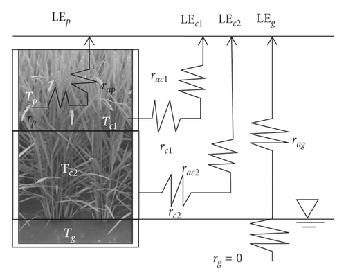
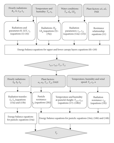
The input data of the three-layer model to estimate T_p include (a) hourly radiations, (b) temperature, humidity, and wind speed, (c) water surface data, and (d) vegetation growth data. T_p was estimated in two steps. The first step was calculating T_c1 and T_c2 by solving heat balance equations with canopy resistances and the second step was estimating T_p with calculated T_c1 and T_c2.

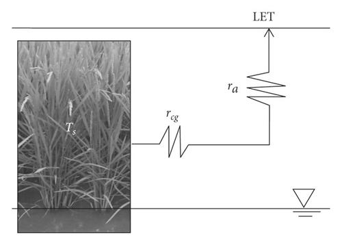
The schematic of the aerodynamic resistance and upper and lower layer canopy resistances of one-layer and three-layer models is illustrated in Figure 1. The schematic diagram illustrating the method for estimation T_c1, T_c2, and T_p by the three-layer model is shown in Figure 2. And the input parameters required for the calculation in the model are shown in Table 1.

Details are in the caption following the image — **Figure 1 (a)**
Open in figure viewer PowerPoint

A schematic representation of the aerodynamic resistance and upper and lower canopy resistances of (a) one-layer and (b) three-layer models. LET was the latent heat flux for the whole canopy (W m⁻²), T_s was the surface temperature of the paddy field (°C), r_a was the aerodynamic resistance to the transfer of sensible heat between the whole rice canopy and water surface (s m⁻¹), r_cg was the total canopy resistance consists of rice canopy resistance and water surface resistance (s m⁻¹), LE_p was the latent heat flux on a panicle (W m⁻²), LE_c1 was the latent heat flux between upper layer rice canopy and atmosphere (W m⁻²), LE_c2 was the latent heat flux between lower layer rice canopy and atmosphere (W m⁻²), LE_g was the latent heat flux between water surface beneath the rice canopy and atmosphere (W m⁻²), T_p was the panicle temperature (°C), T_c1 was the upper layer canopy temperature (°C), T_c2 was the lower layer canopy temperature (°C), T_g was the water temperature (°C), r_ap was the aerodynamic resistance to the transfer of sensible heat between panicle and atmosphere (s m⁻¹), r_ac1 was the aerodynamic resistance to the transfer of sensible heat between upper layer rice canopy and atmosphere (s m⁻¹), r_ac2 was the aerodynamic resistance to the transfer of sensible heat between lower layer rice canopy and atmosphere (s m⁻¹), r_ag was the aerodynamic resistance to the transfer of sensible heat between water surface and atmosphere (s m⁻¹), r_p was the panicle transpiration resistance (s m⁻¹), r_c1 was the upper layer canopy resistance (s m⁻¹), r_c2 was the lower layer canopy resistance (s m⁻¹), and r_g was albedo of water surface (s m⁻¹).

Table 1. Input parameters required for the calculation in the three-layer model.

Symbol	Name	Unit
Forcing parameters
R_n	Net radiation for the whole canopy	W m⁻²
G	Soil heat flux	W m⁻²
L_d	Downward long-wave radiation for the whole canopy	W m⁻²
L_u	Upward long-wave radiation for the whole canopy	W m⁻²
T_a	Air temperature	°C
e_a	Water vapor pressure of the air	hPa
u	Wind speed	m s⁻²

Ground characteristics
T_w	Water temperature	°C
d_w	Water depth	m
LE_g	Latent heat flux between water surface beneath canopy and atmosphere	W m⁻²

Canopy characteristics
a₁	Green leaf and yellow leaf area index in the upper canopy layer	m² m⁻³
a₂	Green leaf and yellow leaf area index in the lower canopy layer	m² m⁻³
PAR	Photosynthetically active radiation	μ mol m⁻² s⁻¹
g_s	Stomatal resistance	cm s⁻¹

Note: g_s was referred to Oue’s literature [32]; other data were observed.

In the one-layer model, the rice canopy and water surface were set as a whole, and energy budget in a paddy field was expressed as follows:

()

where R_n was the net radiation (W m⁻²), LET was the latent heat flux (W m⁻²), H was the sensible heat flux (W m⁻²) for the whole canopy, and δW was the change of storage energy in the water surface (W m⁻²) calculated by equation (2) based on the measured water temperatures and water depth. LET was calculated by the Bowen ratio method (equation 3(a)) with air temperatures and water vapor pressure of air at two different heights, and H was calculated by equation (1). Aerodynamic resistance between the whole rice canopy and water surface (r_a) and the total canopy resistance that consists of rice canopy resistance and water surface resistance (r_cg) was calculated by equations (3b) and (3c):

()

where c_p was the specific heat capacity of the air at constant pressure (J g⁻¹ °C⁻¹), ρ was the air density (kg m⁻³), T_s was the surface temperature of the paddy field (°C), e_sat(T_s) was the saturation-specific humidity at T_s (hPa), and e_a was the specific humidity of the air (kg kg⁻¹).

T_s was the surface temperature of the paddy field (°C) calculated based on the upward long-wave radiation (L_u) and downward long-wave radiation (L_d), as expressed in the following equation:

()

where ε_s was the surface emissivity set as 0.97 in this study.

Based on the data of measured G, δW, LE, and H were calculated by equation (1), and T_s was obtained by equation (4). Subsequently, r_a was obtained by equation (3b), and lastly r_cg was calculated by equation (3c) based on the data of measured T_a, e_a, and LET.

In the three-layer model, net radiation (R_n) sums the net radiation absorbed by upper canopy layer (R_nc1), the net radiation absorbed by lower canopy layer (R_nc2), and the net radiation absorbed by water surface layer (R_ng):

()

The energy budget equations for water surface were written from the following equations:

()

where H_g was the sensible heat flux between water surface beneath canopy and atmosphere (W m⁻²) LE_g was the latent heat flux between water surface beneath canopy and atmosphere (W m⁻²) obtained from the water surface evaporation by the lysimeter, T_g was the ground surface temperature (°C) (assumed T_g = T_w in the model), e_sat(T_g) was the saturation-specific humidity at T_g (hPa), γ was the psychrometric constant (kPa °C⁻¹), r_ag was calculated by equation (7a) based on the measured LE_g and T_g first, H_g was calculated by equation (7b), and then R_ng, R_nc1 + R_nc2 were calculated by equations (5) and (6), respectively.

The energy budget equations for upper canopy layer (50–100 cm) and lower canopy layer (10–40 cm) were written from equations (8) to (10c):

()

where LE_c1 and LE_c2 were the latent heat flux between upper and lower layer canopy and atmosphere (W m⁻²), respectively. H_c1 and H_c2 were the sensible heat flux between upper and lower layer canopy and atmosphere (W m⁻²), respectively. T_c1 was the upper layer canopy temperature (°C), T_c2 was the lower layer canopy temperature (°C), e_sat(T_c1) and e_sat(T_c2) were the saturation-specific humidity at T_c1 and T_c2 (hPa), r_ac1 and r_ac2 were aerodynamic resistances to the transfer of sensible heat between upper and lower layer canopy and atmosphere (s m⁻¹), respectively, r_c1 and r_c2 were the upper and lower layer canopy resistances (s m⁻¹), respectively.

For the aerodynamic resistances, the association of r_a, r_ag, r_ac1, and r_ac2 was expressed in the following equation:

()

In this study, r_c1 and r_c2 were calculated by stomatal resistance (g_s), green leaf and yellow leaf area index in the upper rice canopy layer (a₁), and green leaf and yellow leaf area index in the lower rice canopy layer (a₂), as expressed in equations (12a) and (12b). Because g_s was not measured in the experimental paddy field in 2014, g_s developed by Oue [32] was adopted (values as shown in Table 2), as expressed in equation (13):

()

where g_s was the stomatal conductance (cm s⁻¹), m_s and n_s were parameters, PAR was photosynthetically active radiation (μ mol m⁻² s⁻¹), g_smax was the maximum of stomatal conductance (cm s⁻¹), and g_smin was the minimum of stomatal conductance (cm s⁻¹).

Table 2. m_s and g_smax in the g_s model.

Date	Canopy layer	VPD (hPa)	m_s (cm s⁻¹)/(μ mol m⁻² s⁻¹)	g_smax (cm s⁻¹)
August 6	Upper	∼18	0.00247	1.500
	Upper	18∼	0.00170	0.500
	Lower	∼10	0.002405	1.500
		10∼15	0.002095	1.200
		15∼	0.001925	0.800

August 13	Upper	∼8	0.00780	0.820
	Upper	8∼	0.01246	0.410
	Lower	∼8	0.009935	0.515
	Lower	8∼	0.00833	0.470

August 27	Upper	∼9	0.00282	0.500
	Upper	9∼	0.00195	0.400
	Lower	∼10	0.003155	0.900
		10∼11	0.00261	0.750
		11∼	0.00213	0.450

September 4	Upper	∼16	0.003475	0.550
	Upper	16∼	0.000445	0.400
	Lower	∼15	0.001315	0.400
		15∼16	0.00123	0.400
		∼16	0.00615	0.400

Note: VPD is vapor pressure deficit, g_s is the stomatal conductance (cm s⁻¹), g_smax is the maximum of stomatal conductance (cm s⁻¹), g_smin is the minimum of stomatal conductance (cm s⁻¹), and m_s and n_s are parameters.

With the calculated r_c1 and r_c2, T_c1, T_c2, r_ac1, and r_ac2 were calculated by equations (8)–(10c).

The net radiation input to a panicle (R_in) sums shortwave and long-wave radiation absorbed by the panicle (W m⁻²), as expressed in equation (14a). L_l and L_a were long-wave radiations from a leaf surface adjacent to the panicle and from the atmosphere (W m⁻²), respectively. S_d and S_f were downward direct and diffused shortwave radiations (W m⁻²), respectively, and θ was the solar zenith angle (°), F_p was the inclination factor of panicle, and d_f was the diffusivity factor for radiation. Besides, the heat balance in the panicle layer was written as equation (14b).

()

where F₁ and F₂ were the inclination factors of upper and lower layer rice canopy, respectively. F₁, F₂, and F_p were decided by fitting the calculated transmissivity of downward solar radiation (TDSR) to the measured TDSR (Figure 3).

Besides, H_p and LE_p were sensible and latent heat fluxes on a panicle (W m⁻²), which were written as follows:

()

Moreover, T_ac1 was the air temperature at panicle’s height (°C) which was calculated by the transposition of equation (17) as shown in equation (18a), and likewise, e_ac1 was the absolute humidity at panicle’s height (hPa) calculated as expressed in equation (18b):

()

where r_ap, the aerodynamic resistance to the transfer of sensible heat between panicle and atmosphere (s m⁻¹), denoted the parameter of wind speed (Section 3.3.2), and then r_p, panicle transpiration resistance (s m⁻¹), denoted the parameter of days after the heading stage (Section 3.3.3). Lastly, T_p was calculated by combining equations from equations (14a) to (18b).

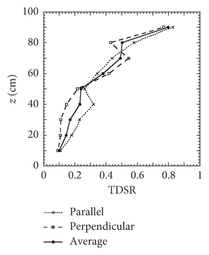
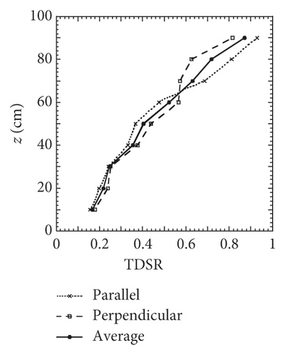
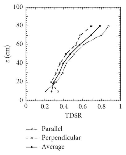
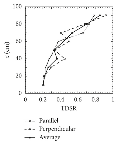
The average value of measured panicle temperature from 50 cm to 100 cm was set as the measured T_p, which was compared with the T_p using the three-layer model and by IM²PACT [30] including the two-layer model.

2.3. Statistical Analysis of Models

The measured and calculated T_c1, T_c2, and T_p were compared by using error analysis and linear regression. Root mean squared error (RMSE), mean absolute error (MAE), and the standard deviation (SD) [33–35] were adopted to evaluate measured and calculated T_c1, T_c2,T_c, and T_p by the models.

2.4. Three-Layer Model Validation

We planted rice (cultivar Hinohikari) from June 21 to November 20, 2015, and rice (cultivar Nikomaru) from June 21 to November 27, 2015, in the same paddy field. PAD of two cultivars was both measured from July 9 to October 14, 2015. Other meteorological instruments were set as same as 2014. Six images were taken to get T_c and T_p by infrared thermometer FLIR-i5 (FLIR systems, USA) at different heights every two or three hours during daytime.

3. Results and Discussion

3.1. General Meteorological Conditions

From July 18 to September 8, the daily average global solar radiation (S_t) was 262 W m⁻², the average air temperature (T_a) was 25°C, while the highest T_a was 35°C on July 26, 2014. The average relative humidity (RH) was 81%, and the average wind speed (u) at 1.0 m reached 0.5 m s⁻¹. The total precipitation, the total evapotranspiration, and the daily evapotranspiration were 670 mm, 567 mm, and 5 mm, respectively.

3.2. Plant Area Density (PAD)

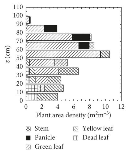
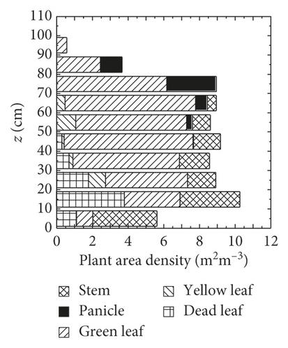
Panicles’ height ranges from 50 cm to 100 cm, and this part of the rice plant was set as the upper canopy layer. There was no panicle on July 18, and the heading was observed on July 25 (Figure 4). The average of the measured green leaf and yellow leaf area index in the upper layer rice canopy (a₁) ranged from 50 cm to 100 cm, which reached its peak on August 8 (2.5) and then decreased. However, green leaf and yellow leaf area index in the lower layer rice canopy (a₂) decreased from 3 on July 25 to 1.5 on August 8, 2014.

3.3. Modeling Parameter Results

3.3.1. Parameters F₁, F₂, and F_p

From August 5 to September 7 in the ripening stage, there was a little diurnal variation of rice morphology.

F₁ was smaller than F₂ because the transmissivity of solar radiation was larger in the upper layer, and the leaf area index of the upper layer canopy (a₁) was also bigger than that in the lower layer (a₂). For example, a₁ was 2.5 and a₂ was 1.5 on August 8. F₁ and F₂ were larger in the morning and afternoon than those at noon, respectively. This was because of the different solar radiation altitudes: in the morning and afternoon, the solar altitude was low, and the solar radiation in the upper layer was large after cutting off, and at noon, the solar radiation was the highest, and the solar radiation in the upper layer was smaller after cutting off. This was dependent on the morphology of canopy: leaves stood upright from 60 cm to 100 cm in the upper layer. In the lower layer, in the morning and afternoon, the solar radiation coming diagonally would be cut off by leaves, while at noon, the solar radiation coming from overhead would not be largely cut off, thereby leading to the smaller F₁ and F₂ during this period.

F_p was important after the ripening stage, when the panicles hung their heads and cover the top of the canopy [36]. F_p variation was similar to that of F₁ from morning to afternoon because of the similar form of panicles and leaves.

F₁ and F₂ were smaller than the leaf inclination factor (F) in the ripening stage published by Maruyama et al. [37]. To estimate the radiation exchange processes in the rice canopy, the hourly variation of F₁, F₂, and F_p should be considered for accuracy.

3.3.2. Aerodynamic Resistance between the Panicle and Atmosphere (r_ap)

Table 3 lists the aerodynamic resistance between the panicle and atmosphere (r_ap) and meteorological data when r_p was set as 0: there was rain before, or dew was found in the morning (August 5, 7, 18, 26, and 28).

Table 3. r_ap in the rice paddy field.

Date	Time	T_p (°C)	T_ac1 (°C)	u (m s⁻¹)	r_ap (s m⁻¹)
August 5	8:30	26.8	27.8	0.4	18.1
August 7	8:30	26.8	28.4	0.6	10.9
August 18	8:30	26.3	26.9	0.6	10.9
August 26	9:30	26.1	27.6	1.7	6.2
August 28	8:30	24.7	25.1	0.6	12.4

Note: r_ap is the aerodynamic resistance to the transfer of sensible heat between panicle and atmosphere, T_p is the panicle temperature, T_ac1 is the air temperature at the panicle’s height, and u is the wind speed.

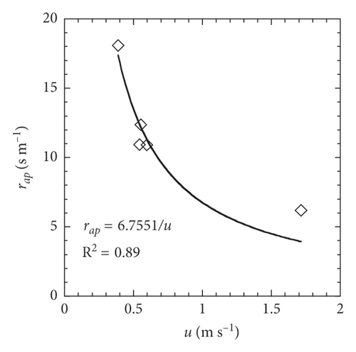
As a result of correlation analysis between the meteorological conditions (S_t, T_a, RH, and u) and r_ap, it was found that r_ap was primarily affected by u with the correlation coefficient of −0.93. This is consistent with the results reported by Yan and Oue [38], which suggested that u at 2.0 m from the ground was the major factor affecting r_a, r_ag, and r_ac (aerodynamic resistance between the rice canopy and atmosphere). The association between u (0.35 m s⁻¹ < u < 1.75 m s⁻¹) and r_ap on the same days is shown in Figure 5(a), as expressed below:

()

The friction of the panicle-atmosphere surface could be weakened by the wind speed, and the transport of heat and water vapor between panicle and atmosphere was primarily attributed to molecular diffusion.

Since from August 5 to September 7, the plant height and PAD only had little difference, and the effect of the canopy structure was not considered for r_ap in this study.

3.3.3. Panicle Resistance for Transpiration (r_p)

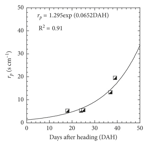
Based on the measured average T_p from 50 cm to 100 cm and r_ap calculated by Eq. (19), r_p can be calculated by equations (16a) and (16b). Five days under large S_t, high T_a and low RH conditions meaning strong transpiration (August 12, 18, 19, and 31 and September 2) were selected to analyze the influence of r_p (Table 4).

Table 4. r_p in the rice paddy field.

Date	Time	DAH	S_t (W m⁻²)	T_a (°C)	u (m s⁻¹)	RH (%)	r_p (s m⁻¹)
August 12	14:30	18	773	29	1.4	70	5.3
August 18	11:10	24	662	31	1.2	68	5.4
August 19	10:30	25	748	33	1.6	60	5.6
August 31	13:00	37	711	29	1.4	65	13.3
September 2	11:30	39	761	29	1.1	67	19.6

Note: DAH is days after heading, S_t is solar radiation, T_a is the air temperature, RH is the relative humidity, u is the wind speed, and r_p is the panicle transpiration resistance.

Correlations between days after heading (DAH), meteorological conditions (S_t, T_a, u, and RH), and r_p suggest that DAH was the major influencing factor, with the correlation coefficient of 0.92. Besides, the changes of r_p against the DAH in the rice paddy field are shown in Figure 5(b). r_p increased asymptotically with the rise in DAH, and their relationship was expressed as follows:

()

Thus far, though there was rare information about r_p, few researchers have measured the transpirational conductance g_p (=1/r_p) in rice paddy fields. Our results showed a similar variation but smaller values compared with those of cultivar “Wuxiangjing 9” reported by Oue et al. [29], in which g_p decreased with the increase in DAH from 0 to 9 under both ambient CO₂ and free air CO₂ enrichment condition.

This new useful method was presented in this study to denote r_p as a parameter by DAH, while some other methods were reported. In the integrated micrometeorology model for panicle and canopy temperature (IM²PACT) developed by Yoshimoto et al. [30], g_p denotes the parameter of the relative humidity in the vicinity of panicle (RH_ac), which was not easily and accurately measured with the ordinary ventilated psychrometers. Based on the measurements of rice varieties at the time of flowering, Fukuoka et al. [39] presented three regression equations of g_p as a function of vapor pressure deficit (VPD).

3.4. Modeling T_p

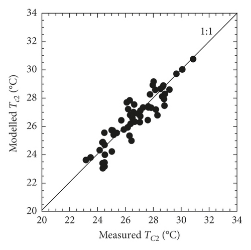
The differences between T_c1 and T_c2 were presented by Wang et al. [40]. The average values of measured canopy temperature from 50 cm to 100 cm and from 10 cm to 40 cm were set as the measured T_c1 and T_c2, which were then compared with the modelled ones, as shown in Figures 6(a) and 6(b). The root mean square errors (RMSE) of modelled T_c1 and T_c2 were 0.76°C and 0.75°C. Besides, the difference between modelled and measured T_c1 and T_c2 ranged from −1.69°C to 1.35°C and from −1.50°C to 1.61°C, respectively. According to results of the 2-tailed t-test statistical analysis, the modelled T_c1 and T_c2 values were not significantly different from the measured values at the 0.05 probability level.

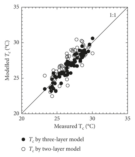
In this study, we set T_c = (T_c1 × a₁ + T_c2 × a₂)/(a₁ + a₂), and measured T_c was compared with that estimated by the two-layer model developed by Yan and Oue [38], as shown in Figure 7(a). RMSE of T_c by our three-layer model was 0.63°C, smaller than that by the two-layer model (1.21°C).

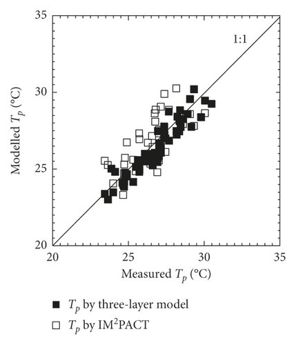
As shown in Figure 7(b), RMSE of T_p estimated by the three-layer model was 0.81°C, smaller than that estimated by IM²PACT (1.27°C) including the two-layer model. Better agreements between the measured and modelled T_p by the three-layer model than that by IM²PACT were obtained, particularly under high T_a conditions as shown in Table 5. This was because (1) T_c1 instead of T_c was used to predict T_p, since modelled T_c1 could be 3°C different with modelled T_c; (2) F₁, F₂, and F_p were determined by fitting the calculated TDSR to the measured TDSR, F₁, F₂, and F_p varied with time because of the different solar radiation altitudes: rather than set to be constant; and (3) r_p denotes the parameter of measured T_p by DAH which considering transpiration cooling instead of the RH_ac.

Table 5. T_p estimated by three-layer model and by IM²PACT [30].

Date	Time	S_t (W m⁻²)	T_a (°C)	RH (%)	T_c (°C)	T_c1 (°C)	T_p by IM²PACT (°C)	T_p by three-layer model (°C)	Mea T_p (°C)
August 5	9:00	212	28	80	26.7	26.2	28.9	26.6	26.8
August 5	14:00	201	30	71	28.1	26.9	27.6	26.9	27.0
August 11	11:00	671	27	73	28.9	25.5	27.0	25.2	25.7
August 18	9:00	235	27	84	26.3	25.8	26.7	26.2	26.3
August 18	12:00	599	31	68	26.8	29.5	27.4	28.4	28.4
August 18	15:00	485	32	68	28.5	26.7	29.7	28.8	28.7
August 19	9:00	477	32	66	28.2	26.1	29.8	28.5	28.9
August 19	14:00	745	32	66	28.5	30.5	28.6	29.6	30.1
August 19	16:00	541	33	59	28.5	28.9	28.5	29.3	29.1
August 20	17:00	188	29	77	28.3	26.4	28.9	27.8	27.7
August 20	18:00	80	29	78	27.7	25.1	27.2	26.5	26.6
August 26	12:00	474	29	67	27.6	26.5	25.7	27.4	27.0
August 26	15:00	442	30	69	28.2	26.4	30.3	27.5	28.1
September 3	15:00	86	29	70	27.2	25.2	29.1	26.5	27.1
September 6	10:00	474	29	71	26.7	24.9	28.1	25.7	26.7
September 6	16:00	93	28	76	29.3	28.8	27.8	30.1	29.3

Note: Mea means measured.

RMSE of T_p estimated by the three-layer model for rice (cultivar Hinohikari) was 0.93°C, and RMSE of T_p estimated by the three-layer model for rice (cultivar Hinohikari) was 0.89°C. Error analysis statistics of the comparison between measured and calculated canopy and panicle temperatures by models is shown in Table 6.

Table 6. Error analysis statistics of the comparison between measured and calculated canopy and panicle temperatures by models.

Temperature	RMSE (°C)	MAE (°C)	SD (°C)
T_c estimated by three-layer model	0.73	0.81	0.64
T_c estimated by two-layer model	1.21	1.56	1.25
T_c1 estimated by three-layer model	0.76	0.75	0.74
T_c2 estimated by three-layer model	0.75	0.63	0.98
T_p estimated by three-layer model	0.81	0.7	0.67
T_p estimated by IM²PCT	1.27	0.95	0.76

Note: T_c is the canopy temperature (°C); two-layer model is developed by Yan and Oue [38]; T_c1 and T_c2 are the upper and lower layer canopy temperatures, respectively; T_p is the panicle temperature (°C); IM²PACT is integrated micrometeorology model for panicle and canopy temperature developed by Yoshimoto et al. [30]; RMSE is the root mean square error, MAE is the mean absolute error, and SD is the standard deviation.

4. Conclusions

Rice panicle temperature (T_p) is a key factor for studying high temperature impacts on spikelet sterility. Comparing with measuring T_p by hand, a T_p simulation model could obtain T_p data readily. We developed the three-layer model to estimate T_p and compared the performance to estimate T_c by three-layer model and T_c by two-layer model developed by Yan and Oue [38]; and to compare the performance to estimate T_p by three-layer model and T_p by IM²PACT [30]. RMSE of T_c by our three-layer model was 0.63°C, smaller than that by the two-layer model (1.21°C). RMSE of T_p estimated by the three-layer model was 0.81°C, smaller than that estimated by IM²PACT (1.27°C).

However, from July 9 to September 8, 2014, there was 29 rainy days, on which T_c1,T_c2, and T_p measurement could not be performed, thereby leading to the reduction of measured data. The highest T_a was 34.64°C on July 26, 2014, and T_c1 and T_p higher than 35.0°C could not be observed, so our model was not used for extreme temperature. Furthermore, the three-layer model simulated fairly well the T_c1, T_c2, and T_p with root mean square errors of 0.76°C, 0.75°C, and 0.81°C, and it was validated well by two other rice cultivars, and thus, it demonstrated that the three-layer model was a new feasible way to estimate T_p. In the future, we will measure stomatal resistance (g_s) in the rice paddy field and analyze the microclimate observational results in the elevated carbon dioxide concentration experiments [41] with different land use [42] to predict T_p.

Disclosure

Hiroki Oue and Zhijun Luo are the co-first authors.

Conflicts of Interest

The authors declare that they have no conflicts of interest.

Acknowledgments

This study was financed in part by the fund “Excellent Engineer” Training Program of General Undergraduate Colleges and Universities in Jiangxi Province: Education and Training Program for Outstanding Engineers in Agricultural Water Conservancy Engineering (Project no. 201442). The authors would like to express their gratitude to Dr. Sanz Grifrio Limin, Ms. Sartika Laban, and Ms. Lian LIU belonging to the hydrometeorology for Environment Engineering Laboratory in Ehime University for their great help in the measurements in the paddy fields. They also thank Mr. Makoto Tanaka and Mr. Kouji Mitsumune from Ehime University Senior High School for supporting our experiments in the paddy fields.

Open Research

Data Availability

The data used to support the findings of this study are available from the corresponding author upon request.

References

1 Horie T., Matsui T., Nakagawa H., and Omasa K., Effect of elevated CO₂ and global climate change on rice yield in Japan, Climate Change and Plant in East Asia. (1996) Springer-Verlag, Tokyo, Japan, 39–56, https://doi.org/10.1007/978-4-431-66899-2_4.
10.1007/978-4-431-66899-2_4
Google Scholar
2 Peng S., Huang J., Sheehy J. E. et al., Rice yields decline with higher night temperature from global warming, Proceedings of the National Academy of Sciences. (2004) 101, no. 27, 9971–9975, https://doi.org/10.1073/pnas.0403720101, 2-s2.0-3042750657.
10.1073/pnas.0403720101
CAS PubMed Web of Science® Google Scholar
3 Wassmann R., Jagadish S. V. K., Sumfleth K. et al., Chapter 3 regional vulnerability of climate change impacts on Asian rice production and scope for adaptation, Advances in Agronomy. (2009) 102, 91–133, https://doi.org/10.1016/s0065-2113(09)01003-7, 2-s2.0-65449185806.
10.1016/S0065-2113(09)01003-7
Web of Science® Google Scholar
4 Nagarajan S., Jagadish S. V. K., Prasad A. S. H. et al., Local climate affects growth, yield and grain quality of aromatic and non-aromatic rice in Northwestern India, Agriculture, Ecosystems & Environment. (2010) 138, no. 3-4, 274–281, https://doi.org/10.1016/j.agee.2010.05.012, 2-s2.0-77955088910.
10.1016/j.agee.2010.05.012
Web of Science® Google Scholar
5 Maruyama A., Weerakoon W. M. W., Wakiyama Y., and Ohba K., Effects of increasing temperatures on spikelet fertility in different rice cultivars based on temperature gradient chamber experiments, Journal of Agronomy and Crop Science. (2013) 199, no. 6, 416–423, https://doi.org/10.1111/jac.12028, 2-s2.0-84886280202.
10.1111/jac.12028
Web of Science® Google Scholar
6 Sathishraj R., Bheemanahalli R., Ramachandran M., Dingkuhn M., Muthurajan R., and Krishna J. S. V., Capturing heat stress induced variability in spikelet sterility using panicle, leaf and air temperature under field conditions, Field Crops Research. (2016) 190, 10–17, https://doi.org/10.1016/j.fcr.2015.10.012, 2-s2.0-85032069516.
10.1016/j.fcr.2015.10.012
Web of Science® Google Scholar
7 Hakata M., Wada H., Masumoto C. et al., Development of a new heat tolerance assay system for rice spikelet sterility, Plant Methods. (2017) 13, 2–8, https://doi.org/10.1186/s13007-017-0185-3, 2-s2.0-85019080209.
10.1186/s13007-017-0185-3
PubMed Web of Science® Google Scholar
8 Kobata T., Palta J. A., Tanaka T. et al., Responses of grain filling in spring wheat and temperate-zone rice to temperature: similarities and differences, Field Crops Research. (2018) 215, 187–199, https://doi.org/10.1016/j.fcr.2017.10.017, 2-s2.0-85033660975.
10.1016/j.fcr.2017.10.017
Web of Science® Google Scholar
9 Wang Y., Wang L., Zhou J. et al., Research progress on heat stress of rice at flowering stage, Rice Science. (2019) 26, no. 1, 1–10, https://doi.org/10.1016/j.rsci.2018.06.009, 2-s2.0-85059086095.
10.1016/j.rsci.2018.06.009
Web of Science® Google Scholar
10 Tian X. H., Luo H. W., Zhou H. D., and Wu C. Y., Research on heat stress on rice in China: progress and prospect, Chinese Agricultural Science Bulletin. (2009) 25, no. 22, 166–168.
Google Scholar
11 Hasegawa T., Ishimura T., Kondo M., Kuwagata T., Yoshimoto M., and Fukuoka M., Spikelet sterility of rice observed in the record hot summer of 2007 and the factors associated with its variation, Journal of Agricultural Meteorology. (2011) 67, no. 4, 225–232, https://doi.org/10.2480/agrmet.67.4.3, 2-s2.0-84969621297.
10.2480/agrmet.67.4.3
Google Scholar
12 Satake T. and Yoshida S., High temperature-induced sterility in indica rices at flowering, Japanese Journal of Crop Science. (1978) 47, no. 1, 6–17, https://doi.org/10.1626/jcs.47.6, 2-s2.0-84996416221.
10.1626/jcs.47.6
Web of Science® Google Scholar
13 Farrell T. C., Fox K. M., Williams R. L., Fukai S., and Lewin L. G., Minimising cold damage during reproductive development among temperate rice genotypes: II—genotypic variation and flowering traits related to cold tolerance screening, Australian Journal of Agricultural Research. (2006) 57, no. 1, 89–100, https://doi.org/10.1071/ar05186, 2-s2.0-31844453852.
10.1071/AR05186
Web of Science® Google Scholar
14 Jagadish S. V. K., Muthurajan R., Oane R. et al., Physiological and proteomic approaches to address heat tolerance during anthesis in rice (Oryza sativa L.), Journal of Experimental Botany. (2010) 61, no. 1, 143–156, https://doi.org/10.1093/jxb/erp289, 2-s2.0-72049121503.
10.1093/jxb/erp289
CAS PubMed Web of Science® Google Scholar
15 Coast O., Murdoch A. J., Ellis R. H., Hay F. R., and Jagadish K. S. V., Resilience of rice (Oryza spp.) pollen germination and tube growth to temperature stress, Plant, Cell & Environment. (2016) 39, no. 1, 26–37, https://doi.org/10.1111/pce.12475, 2-s2.0-84955173403.
10.1111/pce.12475
CAS PubMed Web of Science® Google Scholar
16 Maruyama A., Nemoto M., Hamasaki T., Ishida S., and Kuwagata T., A water temperature simulation model for rice paddies with variable water depths, Water Resources Research. (2017) 53, no. 12, 10065–10084, https://doi.org/10.1002/2017wr021019, 2-s2.0-85036588768.
10.1002/2017WR021019
Web of Science® Google Scholar
17 Nishiyama I. and Blanco L., Avoidance of high temperature sterility by flower opening in the early morning, Japan Agricultural Research Quarterly. (1980) 14, 116–117.
Web of Science® Google Scholar
18 Nishiyama I. and Satake T., High temperature damages in rice plants [Oryza sativa], Japanese Journal of Crop Science. (1981) 25, 14–19.
Google Scholar
19 Baker J. T., Allen L. H., and Boote K. J., Temperature effects on rice at elevated CO₂ concentration, Journal of Experimental Botany. (1992) 43, no. 7, 959–964, https://doi.org/10.1093/jxb/43.7.959, 2-s2.0-0001139529.
10.1093/jxb/43.7.959
Web of Science® Google Scholar
20 Julia C. and Dingkuhn M., Predicting temperature induced sterility of rice spikelets requires simulation of crop-generated microclimate, European Journal of Agronomy. (2013) 49, 50–60, https://doi.org/10.1016/j.eja.2013.03.006, 2-s2.0-84877146770.
10.1016/j.eja.2013.03.006
Web of Science® Google Scholar
21 Zhang Z.-J., Wang Q.-Q., Lang Y.-Z., Wang C.-G., Zhu Q.-S., and Yang J.-C., Effects of high temperature stress at heading stage on pollination and fertilization of different types of rice variety, Acta Agronomica Sinica. (2014) 40, no. 2, 273–282, https://doi.org/10.3724/sp.j.1006.2014.00273, 2-s2.0-85019211900.
10.3724/SP.J.1006.2014.00273
Google Scholar
22 Martínez-Eixarch M. and Ellis R. H., Temporal sensitivities of rice seed development from spikelet fertility to viable mature seed to extreme-temperature, Crop Science. (2015) 55, no. 1, 354–364, https://doi.org/10.2135/cropsci2014.01.0042.
10.2135/cropsci2014.01.0042
Web of Science® Google Scholar
23 Matsui T., Omasa K., and Horie M., The difference in sterility due to high temperatures during the flowering period among japonica-rice varieties, Plant Production Science. (2001) 4, no. 2, 90–93, https://doi.org/10.1626/pps.4.90, 2-s2.0-0034936425.
10.1626/pps.4.90
Web of Science® Google Scholar
24 Abeysiriwardena D. S. D. Z., Ohba K., and Maruyama A., Influence of temperature and relative humidity on grain sterility in rice, Journal of the National Science Foundation of Sri Lanka. (2002) 30, no. 1-2, 33–41, https://doi.org/10.4038/jnsfsr.v30i1-2.2559, 2-s2.0-34248655152.
10.4038/jnsfsr.v30i1-2.2559
Google Scholar
25 Matsui T., Kobayasi K., Nakagawa H. et al., Lower-than-expected floret sterility of rice under extremely hot conditions in a flood-irrigated field in New South Wales, Australia, Plant Production Science. (2014) 17, no. 2, 245–252, https://doi.org/10.1626/pps.17.245, 2-s2.0-84906731420.
10.1626/pps.17.245
Web of Science® Google Scholar
26 Matsui T., Kobayasi K., Yoshimoto M., and Hasegawa T., Stability of rice pollination in the field under hot and dry conditions in the riverina region of New South Wales, Australia, Plant Production Science. (2007) 10, no. 1, 57–63, https://doi.org/10.1626/pps.10.57, 2-s2.0-33846504343.
10.1626/pps.10.57
Web of Science® Google Scholar
27 Tian X. H., Matsui T., Li T. et al., Heat-induced floret sterility of hybrid rice (Oryza sativa L.) cultivars under humid and low wind conditions in the field of Jianghan Basin, China, Plant Production Science. (2010) 13, no. 3, 243–251.
10.1626/pps.13.243
Web of Science® Google Scholar
28 Sheehy J. E., Mitchell P. L., Beerling D. J., Tsukaguchi T., and Ian Woodward F., Temperature of rice spikelets: thermal damage and the concept of a thermal burden, Agronomie. (1998) 18, no. 7, 449–460, https://doi.org/10.1051/agro:19980702, 2-s2.0-0031736792.
10.1051/agro:19980702
Web of Science® Google Scholar
29 Oue H., Yoshimoto M., and Kobayashi K., Effects of free-air CO₂ enrichment on leaf and panicle temperatures of rice at heading and flowering stage, Phyton. (2005) 45, 117–124.
CAS Web of Science® Google Scholar
30 Yoshimoto M., Fukuoka M., Hasegawa T., Utsumi M., Ishigooka Y., and Kuwagata T., Integrated micrometeorology model for panicle and canopy temperature (IM²PACT) for rice heat stress studies under climate change, Journal of Agricultural Meteorology. (2011) 67, no. 4, 233–247, https://doi.org/10.2480/agrmet.67.4.8, 2-s2.0-84865377998.
10.2480/agrmet.67.4.8
Google Scholar
31 Kondo J. and Watanabe T., Studies on the bulk transfer coefficients over a vegetated surface with a multilayer energy budget model, Journal of the Atmospheric Sciences. (1992) 49, no. 23, 2183–2199, https://doi.org/10.1175/1520-0469(1992)049<2183:sotbtc>2.0.co;2.
10.1175/1520-0469(1992)049<2183:SOTBTC>2.0.CO;2
Web of Science® Google Scholar
32 Oue H., Evapotranspiration, photosynthesis and water use efficiency in a paddy field (I)-Stomatal conductance model and single leaf photosynthesis model of rice-, Journal of Japan Society of Hydrology & Water Resources. (2003) 16, no. 4, 375–388, https://doi.org/10.3178/jjshwr.16.375.
10.3178/jjshwr.16.375
Google Scholar
33 Acquah S. J., Yan H. F., Zhang C. et al., Application and evaluation of stanghellini model in the determination of crop evapotranspiration in a naturally ventilated greenhouse, IJABE. (2018) 11, no. 6, 95–103.
Google Scholar
34 Yan H. F., Zhang C., Gerrits M. et al., Parametrization of aerodynamic and canopy resistances for modeling evapotranspiration of greenhouse cucumber, Agriculture and Forest Meteorology. (2018) 262, 370–378, https://doi.org/10.1016/j.agrformet.2018.07.020, 2-s2.0-85050860799.
10.1016/j.agrformet.2018.07.020
Web of Science® Google Scholar
35 Yan H., Acquah S. J., Zhang C. et al., Energy partitioning of greenhouse cucumber based on the application of Penman-Monteith and bulk transfer models, Agricultural Water Management. (2019) 217, 201–211, https://doi.org/10.1016/j.agwat.2019.02.036, 2-s2.0-85062408918.
10.1016/j.agwat.2019.02.036
Web of Science® Google Scholar
36 Oue H., Effects of vertical profiles of plant area density and stomatal resistance on the energy exchange processes within a rice canopy, Journal of the Meteorological Society of Japan. (2001) 79, no. 4, 925–938, https://doi.org/10.2151/jmsj.79.925, 2-s2.0-23044531199.
10.2151/jmsj.79.925
Web of Science® Google Scholar
37 Maruyama A., Kuwagata T., Ohba K., and Maki T., Dependence of solar radiation transport in rice canopies on developmental stage, Japan Agricultural Research Quarterly: JARQ. (2007) 41, no. 1, 39–45, https://doi.org/10.6090/jarq.41.39, 2-s2.0-33947204136.
10.6090/jarq.41.39
Web of Science® Google Scholar
38 Yan H. and Oue H., Application of the two-layer model for predicting transpiration from the rice canopy and water surface evaporation beneath the canopy, Journal of Agricultural Meteorology. (2011) 67, no. 3, 89–97, https://doi.org/10.2480/agrmet.67.3.1, 2-s2.0-84862138147.
10.2480/agrmet.67.3.1
Google Scholar
39 Fukuoka M., Yoshimoto M., and Hasegawa T., Varietal range in transpiration conductance of flowering rice panicle and its impact on panicle temperature, Plant Production Science. (2012) 15, no. 4, 258–264, https://doi.org/10.1626/pps.15.258, 2-s2.0-84867882585.
10.1626/pps.15.258
Web of Science® Google Scholar
40 Wang Y. Y., Oue H., Limin S. G., and Laban S., Effects of water ponding on decreasing leaf and panicle temperature in rice paddy fields, Jurnal Teknologi. (2015) 76, no. 15, 131–137, https://doi.org/10.11113/jt.v76.5965, 2-s2.0-84945288001.
10.11113/jt.v76.5965
Google Scholar
41 Ikawa H., Chen C. P., Sikma M. et al., Increasing canopy photosynthesis in rice can be achieved without a large increase in water use—A model based on free-air CO₂ enrichment, Global Change Biology. (2018) 24, no. 3, 1321–1341, https://doi.org/10.1111/gcb.13981, 2-s2.0-85037996946.
10.1111/gcb.13981
PubMed Web of Science® Google Scholar
42 Yoshida R., Isumi T., Nishimori M. et al., Impacts of land-use changes on surface warming rates and rice yield in Shikoku, western Japan, Geophysical Research Letters. (2012) 39, no. 22, https://doi.org/10.1029/2012gl053711, 2-s2.0-84870612120.
10.1029/2012GL053711
PubMed Web of Science® Google Scholar

Citing Literature

All articles

Estimating Rice Panicle Temperature with Three-Layer Model

Abstract

1. Introduction

2. Materials and Methods

2.1. Measurements in the Rice Paddy Field