Stability and Global Sensitivity Analysis for an Agree-Disagree Model: Partial Rank Correlation Coefficient and Latin Hypercube Sampling Methods
Abstract
In this paper, we present a new mathematical model that describes agree-disagree opinions during polls. We first present the model and its different compartments. Then, we use the next-generation matrix method to compute thresholds of equilibrium stability. We perform the stability analysis of equilibria to determine under which conditions these equilibrium points are stable or unstable. We show that the existence and stability of these equilibria are controlled by the calculated thresholds. Finally, we also perform several computational and statistical experiments to validate the theoretical results obtained in this work. To study the influence of various parameters on these thresholds and to identify the most influential parameters, a global sensitivity analysis is carried out based on the partial rank correlation coefficient method and the Latin hypercube sampling.
1. Introduction
Participation in political life requires citizens’ attention, time, knowledge, money, and motivation. Citizens will participate if they receive benefits commensurate with the cost of participation. Perhaps, the debate on voting is the subject of the most studied political behavior. Individual economic, social, and psychological costs and voting benefits are well known [1]. Candidates and the media often use polls in election campaigns to determine which candidates are in the lead and who are likely to emerge victoriously. Opinion polls are surveys of intent for a sample of voters, while future results allow participants to negotiate and discuss opinions based on a particular outcome. Opinion polls revealed the expected voting quotas. Public opinion polls are widely used to identify people’s political positions, vote, and other behaviors by asking questions about their opinions, activities, and personal characteristics. Answers to these questions are then counted, statistically analyzed, and interpreted. Polls’ result also provides parties with the opportunity to refine their campaign strategies. In the long run, parties change their positions in public opinion [2].
Polls then play a key role in contemporary political campaigns. Party performance updates receive considerable media attention and often serve as a basis for political commentary in the weeks leading up to the election day. We know that knowing the positions of the electorate can affect voter behavior [3, 4]. However, it is unclear how voting shapes party leaders’ strategies during the election campaign. Public opinion is often criticized for influencing voter perceptions and focusing on popularity rather than politics. By strategically communicating the poll results, parties can shape voters’ vision of competition and encourage popular mobilization [5]. This explains why, at the beginning of the 20th century, more than thirty democratic countries banned the publication of opinion polls near elections [6, 7].
To fully understand the role of polls before the elections, it is necessary to take into account the offer of campaigns. This is particularly important in contexts of increased polarization, where holidays play an increasing role in determining the type of information that reaches voters [8]. At any time, party leaders may choose to speak of candidates from their party or other candidates for election, focusing on various political or gender issues. Voter signals in opinion polls can influence party leaders’ decisions to balance these different elements of campaign speech [9].
In the electoral process, where there are only two political parties, the chances of creating strong political polarization are increasing. For example, U. S. citizens face a polarizing scenario during a presidential election, where they must vote for a two-party decision: Republicans and Democrats. Previous studies have shown that U. S. elections are attracting the Internet, where both Twitter and blogs are showing high political polarization [10, 11].
Other political scenarios requiring a bilateral decision are second-round electoral processes. While citizens of the first round can vote from a wide range of different political parties, in the last round, they can vote only for the two final candidates. Voters may not be fully identified with either side, but they still have to take a side. Previous articles have shown that this second round increases political polarization in the country [12]. In [13], the authors analyzed the 2017 presidential election in Chile and measured the resulting political polarization. Of a minority of qualified users, they could estimate the opinion of the majority.
In this contribution, we examine how voters’ preferences and expectations compete with each other when dealing with voter support information to candidates. So, we start by developing a mathematical model to describe the evolution of opinions to predict the probability of results, and then we calculate and analyze the equilibrium points of the model by deriving the important stability thresholds for each equilibrium state.
Through the development of more efficient models, reliable statistical and mathematical methods are needed to improve the accuracy of modeling. One of the most recently popular ways is sensitivity analysis (SA) methods. Sensitivity analysis is used for a variety of reasons, such as developing decisions or recommendations, communicating, understanding or quantifying the system, and developing models. In the development of the model, it can be used to verify the validity or accuracy of the model, to simplify, calibrate, weak process, or lost data, and even to identify the important parameter for other studies [14].
The paper is organized as follows: Section 2 introduces our new model, giving some details about interactions between different compartments and parameters of the model. In Section 3, we derive basic reproduction numbers. Section 4 provides the results of the stability analysis of equilibria. In Section 5, sensitivity analysis is performed to identify the most important parameter in the proposed model, and Section 6 concludes the paper.
2. Presentation of the Model
There are many scenarios involving a binary decision. The poll model that we present here describes the opinions of agreement (or approval) and disagreement (or disapproval), regarding a candidate or idea, in polls preceding the elections. Note that the model can also describe situations in which there are more than two candidate parties because we can always reduce the situation to two decisions. For example, if there are four parts A, B, C, and D, we wish to study the political position of party A, and we can then examine the two subsets {A} and {B, C, D} of the investigation. Votes for A are considered agree, and votes for B, C, or D are considered disagree. More simply, we consider the opinion poll of voters on the performance of the party studied. As an example, we can cite the “approve or disapprove” poll done by Thomson Reuters on how Donald Trump fulfills his role as the president [15].
Without loss of generality, we devise a mathematical model describing the evolution of agree and disagree opinions during polls (surveys), and the types of surveys we consider here are surveys that can be answered in agreement, disagreement, or otherwise. Thus, the population targeted by the poll is regrouped into three groups: agree, disagree, and ignorant individuals.
- (1)
Ignorant (I): people who do not know about the poll or those who abstain from voting for personal reasons
- (2)
Agree (A): people in agreement with the idea being studied
- (3)
Disagree (D): people in disagreement with the idea being studied
- (1)
The targeted population is well mixed, that is, the ignorant individuals are homogeneously spread throughout the population
- (2)
Recruitment and mortality are negligible under the temporal scale consideration; therefore, no individual is recruited and no individual dies during the poll
- (3)
Individuals have the right to communicate with each other and can thus convince one another
- (4)
People who are unsure of their opinion are ignorant
- (5)
People who abstain from voting are ignorant
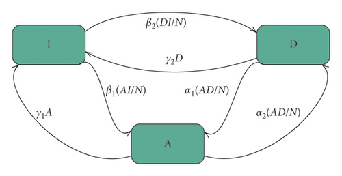
Everyone has their reasons for agreement or disagreement. An ignorant person can be persuaded by someone who agrees at a rate β1 or by someone who does not agree with the opinion at a rate β2. A person agreeing with the opinion may be persuaded by someone who does not agree at a rate α2, or a person who disagrees with the opinion may be persuaded by someone who agrees at a rate α1. People can abstain from voting or lose interest without any direct contact with individuals from the opposite opinion group, then agree people become ignorants at the rate γ1, and disagree people become ignorants at the rate γ2. A flowchart describing different interactions between the compartments of the model is presented in Figure 1.
Therefore, all the solutions of systems (1)–(3) are nonnegative.
A summary of parameter description is given in Table 1.
| Parameter | Description |
|---|---|
| β1 | Ignorant to agree transmission rate |
| β2 | Ignorant to disagree transmission rate |
| α1 | Disagree to agree transmission rate |
| α2 | Agree to disagree transmission rate |
| γ1 | Interest loss factor of agree individuals |
| γ2 | Interest loss factor of disagree individuals |
3. Thresholds: Basic Reproductive Numbers
In epidemiology, the basic reproductive number R0 (or epidemic threshold) is defined as the average number of secondary cases of an infection produced by a “typical” infected individual during his/her entire life as infectious when introduced in a population of susceptibles [17–21]. The threshold R0 is mathematically characterized in terms of infection transmission as a “demographic process,” but offspring production is not seen as giving birth in a demographic sense, but it causes new infections through transmission [22–24]. Thus, the infection process can be considered as a “consecutive generation of infected individuals.” The following growing generations indicate a growing population (i.e., an epidemic), and the growth factor for each generation indicates the potential for growth. So, the mathematical characterization of R0 is this growth factor [22]. Generally, if R0 > 1, an epidemic occurs, whereas if R0 < 1, there will probably be no epidemic.
Following this definition, we will define our thresholds as follows: RD0 is the average number of new disagreements produced by an individual disagreeing introduced in a population of ignorant people during the period in which he or she was in this opinion. And, RA0 is the average number of new agreements produced by an individual in agreement and that was introduced into a population of ignorant people during the period in which he or she was in that opinion.
For the analysis of epidemic models, the first step is to calculate the disease-free equilibrium (DFE). This equilibrium point is then used to calculate the basic reproductive number using the next-generation matrix method. The objective of this section is only the calculation of the thresholds and not the equilibrium states of the model. But, in this method, we have to determine the equilibrium states when A = 0 and when D = 0.
In this contribution, let RX0 be the threshold of growing of the opinion X (either X = A “agree” or X = D “disagree”). Then, RD0 is the threshold associated with the disagree-free equilibrium, while RA0 is the one associated with the agree-free equilibrium.
We calculate the equilibria for the aforementioned model, and based on the next-generation matrix approach, we derive associated thresholds.
4. Stability Analysis
4.1. Steady States
This system has four equilibrium points, and the trivial equilibrium E0 = (0,0) is an equilibrium that exists always without any condition. It means there is no survey and there is no need to opinions.
One disagree-free equilibrium E1 = (1 − (γ1/β1), 0) exists if the condition β1 > γ1 holds, and the agree-free equilibrium E2 = (0,1 − (γ2/β2)) exists if β2 > γ2 holds.
Thus, from (25), we deduce that a∗ > 0 and d∗ > 0. Throughout the article and without loss of generality, we just consider the first condition as a sufficient condition for the existence of E∗.
4.2. Stability of Steady States
Proposition 1. The equilibrium E0 = (0,0) is unstable if β1 > γ1 or β2 > γ2. Otherwise, it is stable.
Proof. The Jacobian matrix at this equilibrium is
It is clear that if β1 > γ1 or β2 > γ2, we get one positive eigenvalue of J(E0), and then E0 is unstable. Else, we have all eigenvalues of J(E0) having the negative real part, which completes the proof.
Remark 1. Note that the conditions in the previous proposition imply the existence of E1 or E2. Therefore, E0 is unstable whenever there exists E1 or E2.
Proposition 2. The equilibrium E1 = (1 − (γ1/β1), 0) is unstable if RD0 > 1. Otherwise, it is stable.
Proof. The Jacobian matrix at this equilibrium is
The eigenvalues of J(E1) are
It is clear from the existence condition of this equilibrium that γ1 − β1 < 0. Thus, the stability of the point of equilibrium E1 is based on the eigenvalue λ2 of the matrix J(E1). By a simple calculation, we have
This implies that if RD0 > 1, E1 is unstable; else, E1 is stable.
Proposition 3. The equilibrium E2 = (0,1 − (γ2/β2)) is unstable if RA0 > 1. Otherwise, it is stable.
Proof. The Jacobian matrix at this equilibrium is
The eigenvalues of J(E2) are
It is clear from the existence condition of this equilibrium that γ2 − β2 < 0. Thus, the stability of the point of equilibrium E2 is based on the eigenvalue λ1 of the matrix J(E2). By a simple calculation, we have
This implies that if RA0 > 1, E2 is unstable; else, E2 is stable.
Proposition 4. The equilibrium E∗ = (a∗, d∗), where
Proof. The Jacobian matrix at this equilibrium is
Using fact (23), we have
Then,
By the conditions “β1 < γ1 and γ2 < β2 and α > 0” or “β1 > γ1 and γ2 > β2 and α < 0,” we have −(β1γ2 − β2γ1/α) > 0, and by existence conditions and
Remark 2. (1) Note that the conditions RD0 > 1 and RA0 > 1 lead to the instability of E1 and E2 and help in the existence of E∗.
(2) Sufficient conditions in the above proposition could be reduced to α (β1γ2 – β1γ2) < 0.
A summary of sufficient existence and stability conditions of the steady states of model (11) is given in Table 2.
| Equilibrium | Existence conditions | Stability conditions |
|---|---|---|
| E0 | — | β1 < γ1 and β2 < γ2 |
| E1 = (1 − (γ1/β1), 0) | β1 > γ1 | RD0 < 1 |
| E2 = (0,1 − (γ2/β2)) | β2 > γ2 | RA0 < 1 |
| E∗ = (a∗, d∗) | RD0 > 1 and RA0 > 1 and α(α − β1 + β2) > 0 | β1 < γ1 and γ2 < β2 and α > 0 or β1 > γ1 and γ2 > β2 and α < 0 |
4.3. Examples
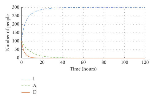
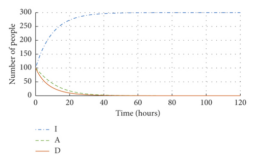
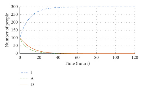
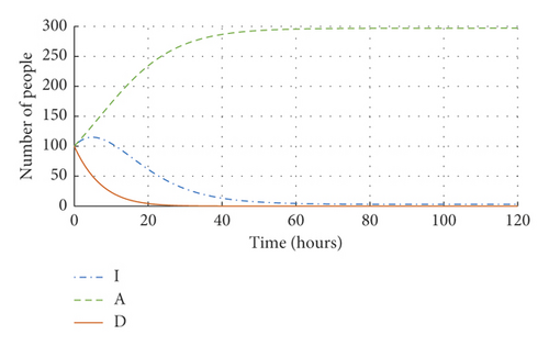
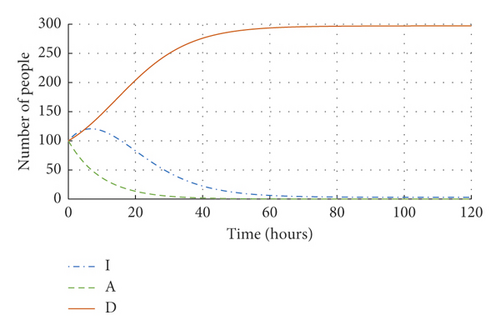
It can be seen from Table 3 that the equilibrium E0 exists and it is stable in the four cases: example 1: RD0 > 1 and RA0 > 1, example 2: RA0 < 1 and RD0 < 1, example 3: RD0 < 1 and RA0 > 1, and example 4: RD0 > 1 and RA0 < 1.
| β1 | β2 | α1 | α2 | γ1 | γ2 | RD0 | RA0 | ||
|---|---|---|---|---|---|---|---|---|---|
| 1 | E0 = (300,0,0) | 0.0010 | 0.1010 | 0.1010 | 0.3010 | 0.5010 | 0.3010 | 1.9901 | 2.0730 |
| 2 | E0 = (300,0,0) | 0.0010 | 0.2010 | 0.2010 | 0.3010 | 0.1010 | 0.5010 | 0.5000 | 0.8543 |
| 3 | E0 = (300,0,0) | 0.0010 | 0.0010 | 0.2010 | 0.1010 | 0.1010 | 0.1010 | 0.5000 | 2.0001 |
| 4 | E0 = (300,0,0) | 0.0010 | 0.0010 | 0.1010 | 0.2010 | 0.1010 | 0.1010 | 2.0001 | 0.5000 |
| 5 | E1 = (2.9703, 297.0297, 0) | 0.1010 | 0.0010 | 0.2010 | 0.2010 | 0.0010 | 0.0010 | 0.6634 | 0.4925 |
| 6 | E1 = (2.9703, 297.0297, 0) | 0.1010 | 0.0010 | 0.0010 | 0.0010 | 0.0010 | 0.0010 | 0.5025 | 101 |
| 7 | E2 = (2.9703, 0,297.0297) | 0.0010 | 0.1010 | 0.2010 | 0.2010 | 0.1010 | 0.0010 | 0.4925 | 0.6634 |
| 8 | E2 = (2.9703, 0,297.0297) | 0.0010 | 0.1010 | 0.0010 | 0.0010 | 0.0010 | 0.0010 | 101 | 0.5025 |
| 9 | 0.5010 | 0.1010 | 0.1010 | 0.0010 | 0.2010 | 0.0010 | 0.6688 | 0.5196 | |
| 10 | 0.1010 | 0.5010 | 0.0010 | 0.1010 | 0.0010 | 0.2010 | 0.5196 | 0.6688 | |
| 11 | E∗ = (133.3333, 10.5556, 156.1111) | 0.1010 | 0.7010 | 0.3010 | 0.0010 | 0.2010 | 0.3010 | 467.7774 | 1.0672 |
| 12 | E∗ = (214.2857, 80.4643, 5.2500) | 0.3010 | 0.4010 | 0.0010 | 0.8010 | 0.2010 | 0.5010 | 1.0649 | 300.8004 |
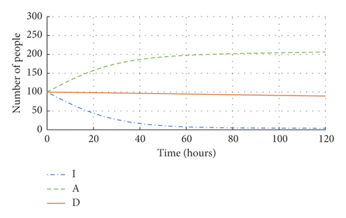
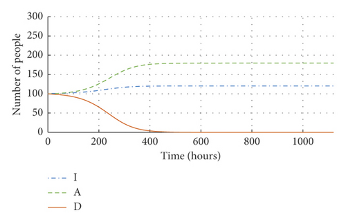
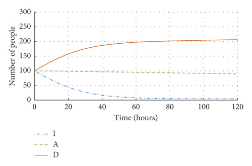
Example 5 shows the existence and the stability of the steady state E1 in the case of RA0 < 1 and RD0 < 1 and in the case of RA0 > 1 and RD0 < 1 in example 6. Examples 7 and 8 show the existence and the stability of the equilibrium E2 in the cases of “RA0 < 1 and RD0 < 1” and “RA0 < 1 and RD0 > 1,” respectively.
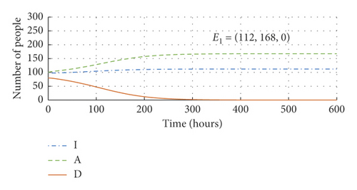
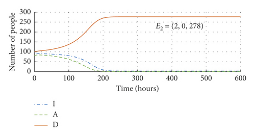
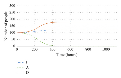
Examples 9 and 10 show the possibility of the existence and stability of the two steady states E1 and E2 at the same time, that is, “β1 > γ1 and β2 > γ2 and RA0 < 1 and RD0 < 1.” These examples give an insight about the stability of each equilibrium for given parameters’ values. After some numerical calculations, we noted that, in this situation, the parameters γ1 and γ2 may switch from E1 to E2 and the inverse, while if γ1 > γ2, then E1 will be more attractive, and if γ2 > γ1, then E2 will be more attractive and that with the same initial conditions. We simulate the model with different initial conditions to illustrate the impact of initial conditions on the stability of E1 and E2 in this situation. Figure 2 depicts the stability of E1 and E2 at the same time, where we consider the same set of parameters from example 9 in Table 3. By changing the initial conditions, we can see that E1 is stable when I(0) = 100, A(0) = 100, and D(0) = 80, while it can be seen that E2 is also stable with this set of parameters but after choosing I(0) = 100, A(0) = 80, and D(0) = 100.
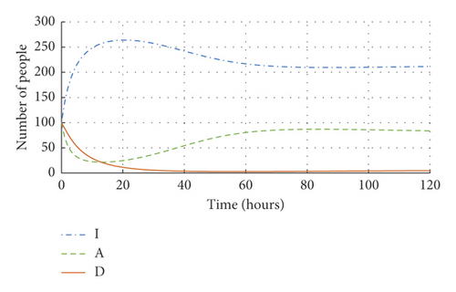
Example 11 shows the existence and the stability of the equilibrium E∗, where “RD0 > 1 and RA0 > 1 and α(α − β1 + β2) > 0” and “β1 < γ1 and γ2 < β2 and α > 0,” while example 12 shows the existence and the stability of E∗, where “RD0 > 1 and RA0 > 1 and α(α − β1 + β2) > 0” and “β1 > γ1 and γ2 > β2 and α < 0.”
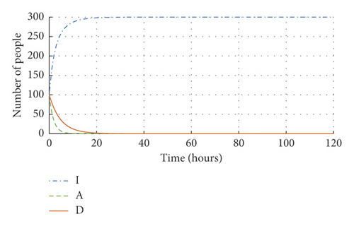
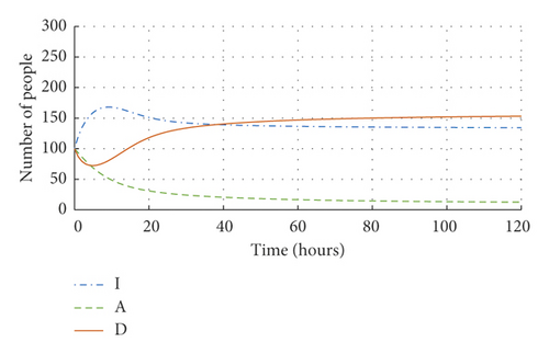
Figure 3 depicts examples of the existence and stability of the equilibrium state E0 for different parameters’ values and threshold RD0 and RA0 values simulated with initial conditions and parameters’ values from Table 3. Figure 4 depicts examples of the existence and stability of the equilibrium state E1 for different parameters’ values and threshold RD0 and RA0 values simulated with initial conditions and parameters’ values from Table 3. It can be seen from Figure 4(b) that the function D decreases towards zero, but it will take a long time. In the Figure 4(c), we have considered 1,200 hours to show that the function D will go to zero but very slowly. Figure 5 depicts examples of the existence and stability of the equilibrium state E2 for different parameters’ values and threshold RD0 and RA0 values simulated with initial conditions and parameters’ values from Table 3. We can see from Figure 5(b) that the function A will also take a very long time to go to zero. In Figure 5(c), we have considered 1,200 hours to show that function A will tend to zero but very slowly. Figure 6 depicts examples of the existence and stability of the equilibrium state E∗ for different parameters’ values and threshold RD0 and RA0 values simulated with initial conditions and parameters’ values from examples 11 and 12 of Table 3.
5. Analysis of Thresholds
5.1. No Abstention: No Loss of Interest
E1 exists without any condition, and it is stable if α2 < α1, and E2 exists without any condition, and it is stable if α1 < α2.
This result explains the effect of the polarization on the outcome of polls. When there is no abstention from voting and people keep their interest in voting, then the most influential parameters on the outcome of the polls are the polarization factors α1 and α2. For example, during a poll determining the political position of one candidate Y by voting with Approve or Disapprove or otherwise, if candidate Y can convince people by his political vision and/or by other ways, then he can change the course of events in his favor. Mathematically, he makes α2 < α1. But, if somehow he contributes to making α1 < α2, then things could spin out of control on the election day.
5.2. One Chance
5.3. Statistical Analysis
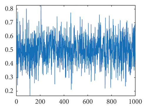
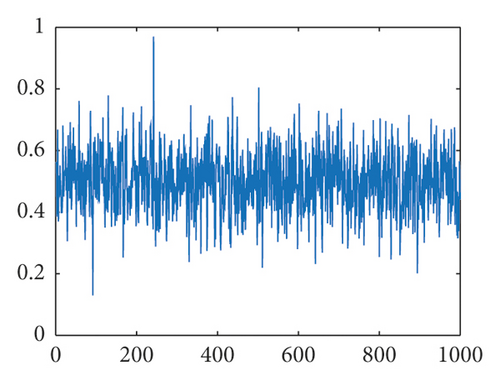
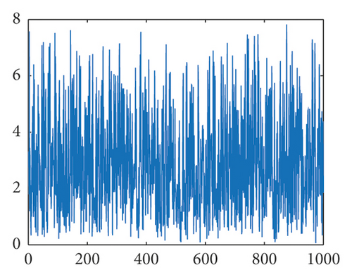
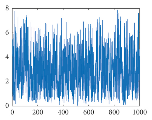
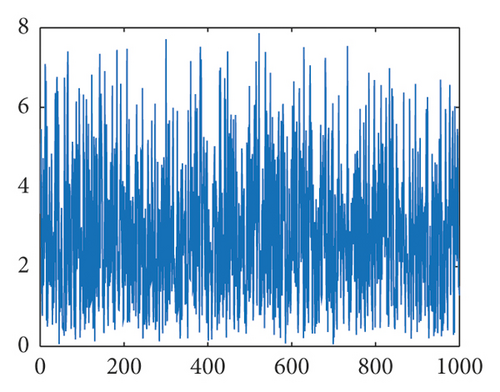
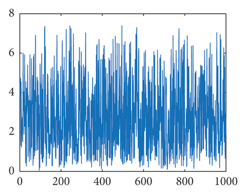
Here, we use probability distribution functions of the six parameters given in Table 4 sampled by using the Latin hypercube sampling, see Figure 7. We compute the probabilities of equilibria existence and stability conditions. It can be seen from Table 5 that the probability of E1 to exist is about 0.5960, while its probability of stability is about 0.53. The probability of E1 to exist and to be stable is 0.4040. The probability of the existence of E2 is about 0.6250, while the probability of its stability is about 0.5370. The probability of E1 to exist and to be stable is 0.43. The equilibrium E∗ has a probability of existence about 0.0240 and a probability of stability about 0.2190, while E∗ exists, and it is stable with a probability of 0.001.
| Parameters | |
|---|---|
| β1 | Normal |
| β2 | Normal |
| α1 | Triangular |
| α2 | Triangular |
| γ1 | Triangular |
| γ2 | Triangular |
| Equilibrium | Probability of existence | Probability of stability | Probability of existence and stability |
|---|---|---|---|
| E1 | 0.5960 | 0.5300 | 0.4040 |
| E2 | 0.6250 | 0.5370 | 0.4300 |
| E∗ | 0.0240 | 0.2190 | 0.001 |
6. Sensitivity Analysis
Global sensitivity analysis (GSA) approach helps to identify the effectiveness of model parameters or inputs and thus provides essential information about the model performance. Out of the many methods of carrying out sensitivity analysis is the partial rank correlation coefficient (PRCC) method that has been used in this paper. The PRCC is a method based on sampling. One of the most efficient methods used for sampling is the Latin hypercube sampling (LHS), which is a type of Monte Carlo sampling [25] as it densely stratifies the input parameters. As the name suggests, the PRCC measures the strength between the inputs and outputs of the model using correlation through the sampling done by the LHS method [26–28].
Parameters β1 and β2 follow normal distribution with mean and standard deviation 0.5 and 0.01, respectively, while parameters α1, α2, γ1, and γ2 follow triangular distribution with minimum, maximum, and mode as 0.02, 0.8, and 0.51, respectively. A summary of probability distribution functions is given in Table 4. In Latin hypercube sampling approach, probability density function (given in Table 4) for each parameter is stratified into 100 equiprobable (1/100) serial intervals. Then, a single value is chosen randomly from each interval. This produces 100 sets of values of RD0 and RA0, from 100 sets of different parameter values mixed randomly, calculated by using equations (4) and (5), respectively.
Sensitivity analysis has been done concerning the basic reproduction numbers RD0 and RA0, and the main objective of this section is to identify which parameters are important in contributing variability to the outcome of basic reproduction numbers based on their estimation uncertainty.
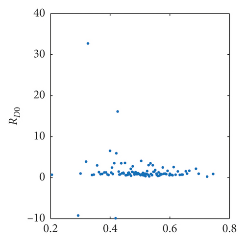
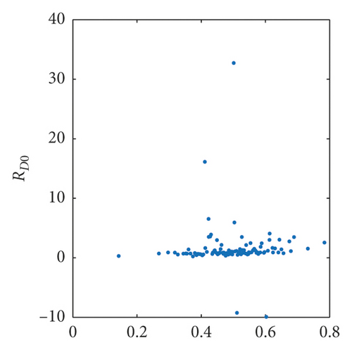
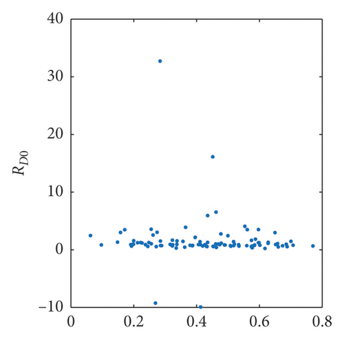
To sort the model parameters according to the size of their effect on RD0 and RA0, a partial rank correlation coefficient is calculated between the values of each of the six parameters and the values of RD0 and RA0 in order to identify and measure the statistical influence of any one of the six input parameters on thresholds RD0 and RA0. The larger the partial rank correlation coefficient, the larger the influence is on the input parameter affecting the magnitude of RD0 and RA0.
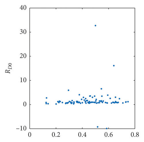
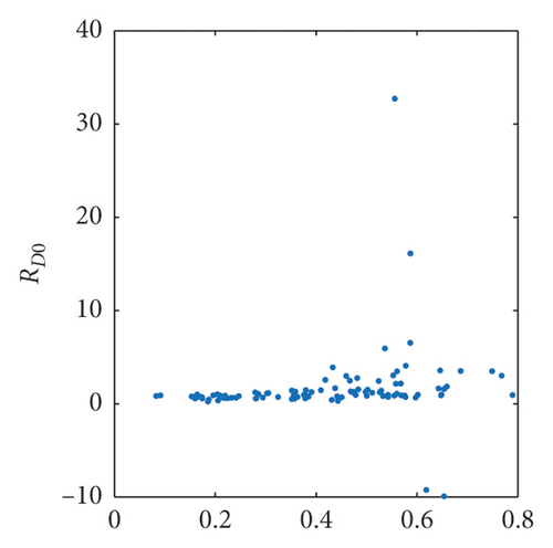
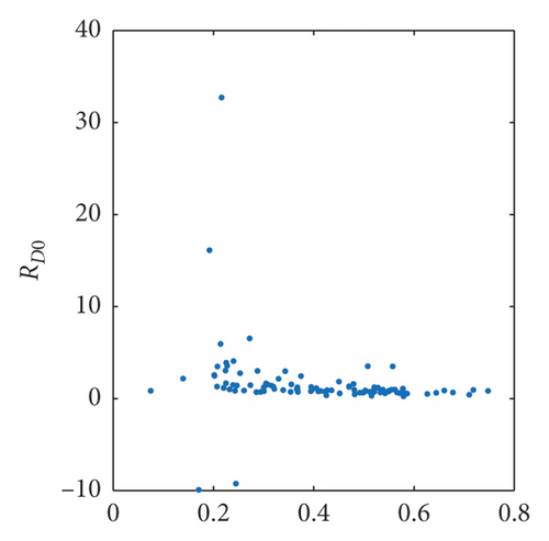
As shown in Table 6, the transmission rate, β1, and parameters γ1 and γ2 are highly correlated with the threshold RD0 with corresponding values −0.1374 and 0.1613 and −0.2101, respectively. Moderate correlation exists between transmission rates α1 and α2 and RD0 with corresponding values as −0.0633 and 0.0669, respectively. Weak correlations have been observed between the transmission rate β2 and RD0 with the corresponding value 0.0025.
| Parameters | Sampling | PRCCs | p value | Sensitivity index |
|---|---|---|---|---|
| β1 | LHS | −0.1374 | 0.1728 | 0.5596 |
| β2 | LHS | 0.0025 | 0.9800 | 0.0192 |
| α1 | LHS | −0.0633 | 0.5318 | 0.1065 |
| α2 | LHS | 0.0669 | 0.5085 | 0.5269 |
| γ1 | LHS | 0.1613 | 0.1090 | 0.7492 |
| γ2 | LHS | −0.2101 | 0.0359 | 0.8499 |
As shown in the sensitivity index column of Table 6, the parameter γ2 accounts for the maximum variability 0.8499 in the outcome of basic reproduction number RD0. The parameter γ1 is the next to account for the variability 0.7492 in the outcome of RD0. Then, the transmission rate β1 accounts for the variability 0.5596 in the outcome of RD0 followed by the transmission rate α2 that accounts for the variability 0.5269 in the outcome of RD0. Transmission parameters α1 and β2 account for the least variability 0.1065 and 0.0192 in the outcome of basic reproduction number RD0, respectively. Hence, parameters γ1 and γ2 and the transmission rate β1 are the most influential parameters in determining RD0.
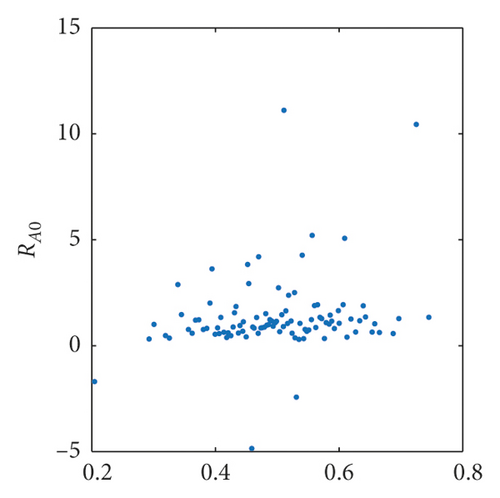
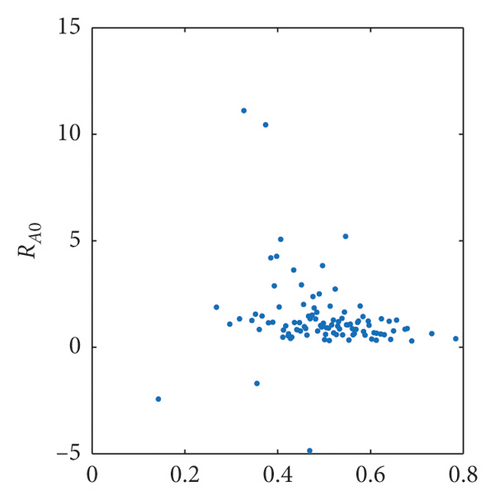
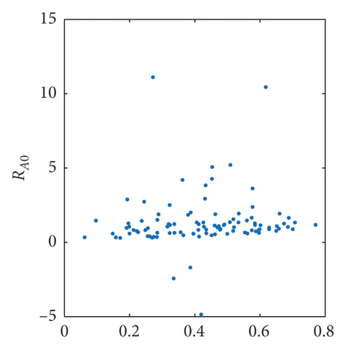
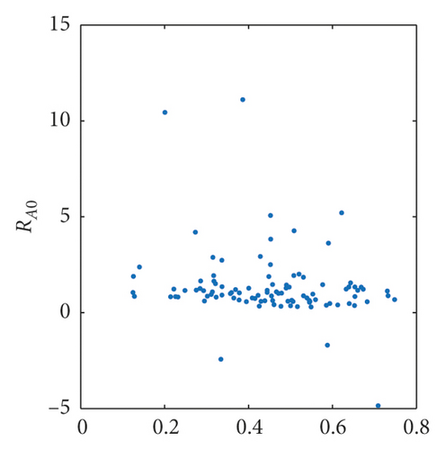
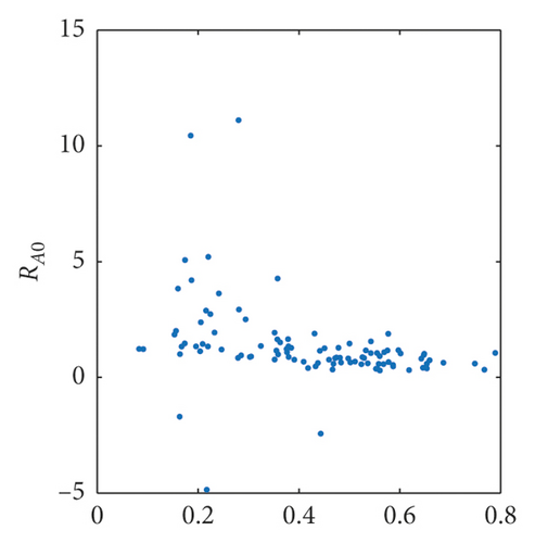
It can be seen from Table 7 that the parameter γ1 is highly correlated with the threshold RA0 with the corresponding value −0.3343. Moderate correlation exists between transmission rates β1, β2, and α2 and the parameter γ2 and RA0 with corresponding values as 0.2137, −0.1928, −0.2076, and 0.2523, respectively. Weak correlations have been observed between the transmission rate α1 and RA0 with the corresponding value 0.0857.
| Parameters | Sampling | PRCCs | p value | Sensitivity index |
|---|---|---|---|---|
| β1 | LHS | 0.2137 | 0.0328 | 0.5753 |
| β2 | LHS | −0.1928 | 0.0546 | 0.2421 |
| α1 | LHS | 0.0857 | 0.3967 | 0.0159 |
| α2 | LHS | −0.2076 | 0.0382 | 0.3872 |
| γ1 | LHS | −0.3343 | 6.7425e−04 | 0.8004 |
| γ2 | LHS | 0.2523 | 0.0113 | 0.7122 |
One can see in the sensitivity index column of Table 7 that the parameter γ1 accounts for the maximum variability 0.8004 in the outcome of basic reproduction number RA0. The parameter γ2 is the next to account for the variability 0.7122 in the outcome of RA0. The transmission rate β1 accounts for the variability 0.5753 in the outcome of this threshold followed by the transmission rate α2 that accounts for the variability 0.3872 in the outcome of RA0. Transmission parameters β2 and α1 account for the least variability 0.2421 and 0.0159 in the outcome of basic reproduction number RA0, respectively. Hence, parameters γ1 and γ2 and the transmission rate β1 are also the most influential parameters in determining RA0.
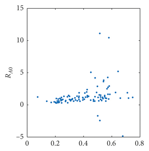
Scatter plots comparing the basic reproduction numbers RD0 and RA0 against each of the six parameters: β1, β2, α1, α2, γ1, and γ2 are shown in Figures 8 and 9, respectively, based on Latin hypercube sampling with a sample size of 100. These scatter plots clearly show the linear relationships between outcome of RD0 and RA0 and input parameters.
7. Conclusion
In this paper, an IAD model-type compartmental model has been considered to explore agree-disagree opinions during polls. The equations governing the system have been solved to compute equilibrium states, and the next-generation matrix method is used to derive basic reproduction numbers RA0 and RD0.
The model exhibits four feasible points of equilibrium, namely, the trivial equilibrium, agree-free equilibrium, disagree-free equilibrium, and the positive equilibrium. Sufficient equilibrium conditions of existence are given, and stability analysis is performed to show under which conditions equilibrium states are stable or unstable. The stability of these points of equilibrium is controlled by the threshold number RA0 and RD0. If the threshold, RD0, is less than one, the disagree opinion dies out and the disagree-free equilibrium is stable. If RD0 is greater than one, the disagree opinion persists and the disagree-free equilibrium is unstable. If the threshold, RA0, is less than one, the agree opinion dies out and the agree-free equilibrium is stable. If RA0 is greater than one, the agree opinion persists and the disagree-free equilibrium is unstable. We simulated some examples with different parameter values to show the existence and the stability of such equilibria.
The probabilities of the existence and probabilities of the stability of equilibria are computed based on the parameters’ distribution function sampled with the Latin hypercube sampling method. To identify the most influential parameter in the proposed model, global sensitivity analysis is carried out based on the partial rank correlation coefficient method and Latin hypercube sampling. This statistical study shows that the most influential parameters in the determination of thresholds of equilibria stability are β1, the polarization parameter of ignorant people by people agreeing, the parameter, γ1, of the loss of interest of the people agreeing, and finally γ2, the parameter of loss of interest of disagreeing people.
Conflicts of Interest
The authors declare that they have no conflicts of interest.
Acknowledgments
The authors would like to thank all the members of the Editorial Board who were responsible for this paper.
Open Research
Data Availability
No data were used to support this study.


