Many engineering systems change appreciably over a relatively short time interval due to their fast evolution in the dynamics. Time-varying (TV) system’s ambient excitation is usually difficult to measure under operating conditions, and its dynamics have to be determined without measuring the excitation. Therefore, short data-based output-only identification for TV systems with fast dynamic evolution is considered in this paper. Deterministic parameter evolution methods are known to track fast dynamic evolution by postulating TV model parameters as deterministic functions of time and selecting proper functional subspaces. However, these methods require a significant number of parameters to represent complicated time-dependencies and dynamics characterized by larger numbers of degrees-of-freedom. In such cases, the ordinary least squares estimation may lead to less accurate or even unreliable estimates. A ridge regression-based deterministic parameter evolution method is proposed to overcome ill-posed problems via regularization and subsequently assessed through numerical and experimental validation. Comparative results confirm the advantages of the proposed method in terms of achievable natural frequency and power spectral density tracking, accuracy, and resolution of TV systems with fast dynamic evolution, when the response data length is relatively short.

1. Introduction

The need for time-varying (TV) system characterization is pervasive throughout the aerospace, mechanical, transportation, and manufacturing engineering practice. It is usually difficult to build the explicit dynamic model of a practical system via mechanism analysis; hence, TV system identification in a way that takes time variation explicitly into account is receiving more and more attention [1–4]. With the development of engineering applications, systems with fast varying dynamics are being widely used and their intrinsic nonstationary characteristics are increasingly inevitable. On the one hand, these systems may change appreciably over a relatively short time interval due to their fast evolution in the dynamics. On the other hand, the dynamic characteristics of TV systems may not fit into a laboratory and controlled testing may not be feasible under operating conditions. In other words, TV system’s ambient excitation is usually difficult to measure under operating conditions and its dynamics have to be determined without measuring the excitation. Therefore, short data-based output-only identification for TV systems is considered in this work in order to capture their fast varying dynamics.

Identification methods for TV systems are generally classified under the umbrella of time-frequency methods [1]. Most frequency-domain methods employ time-frequency analysis (e.g., the short time Fourier transform, Cohen’s class, wavelet-based methods, the Hilbert–Huang transform, etc.), which are based on nonparametric representations of the nonstationary signal as a simultaneous function of time and frequency. By contrast, time-domain methods employ parametric representations (e.g., time-dependent autoregressive moving average (TARMA) models), which offer a number of potential advantages, such as improved accuracy, resolution, and tracking of the TV dynamics. TARMA model-based methods may be further divided into three classes according to the type of “structure” imposed upon the evolution of the TV model parameters: unstructured parameter evolution (UPE), stochastic parameter evolution (SPE), and deterministic parameter evolution (DPE) methods [3]. The DPE methods are mainly based on explicit models of parameter evolution through projecting the parameter trajectory onto specific functional subspaces defined by deterministic basis functions (such as trigonometric, Legendre, Chebyshev, wavelets, B-splines, moving Kriging shape functions, radial basis functions, and others). By postulating TV model parameters as deterministic functions of time, the TARMA model can be transformed into a functional series (FS) TARMA model with time-invariant parameter matrix. Therefore, DPE methods are known to track fast dynamic evolution by selecting proper functional subspaces over their UPE and SPE counterparts [2–4].

DPE methods have played an important role in the development of TV system identification and nonstationary signal processing. In 1970, Rao [5] approximated AR coefficients by truncated Taylor series expansion and introduced the idea of representing TV model parameters as polynomials of time. Thereafter, Mendel [6] summarized the nonstationary identification methods and classified them into UPE, SPE, and DPE, which are still in use today. Kozin [7] approximated AR coefficients by a linear combination of Legendre basis functions and applied the FS-TAR model to earthquake ground motion analysis. In 1983, Grenier [8] extended the FS-TAR model to the FS-TARMA case by examining the existence and uniqueness of a FS-TARMA model representation for a nonstationary system, which was successfully applied to speech signal modeling [9–12]. Gersh and Kitagawa [13] extended the univariate FS-TAR model to the multivariate/vector case. Niedzwiecki [14, 15] defined the idea of expanding TV model parameters onto linear combinations of basis functions as “functional series modeling” and proposed a recursive least squares for the estimation of FS-TAR model parameters. Tsatsanis and Giannakis [16, 17] proposed FS-TARMA models with exogenous input and FS time-dependent finite impulse response models and considered the issue of model structure selection. In 2000, Niedzwiecki [2] summarized the DPE methods and investigated the time and frequency characteristics of basis function estimators.

In 2006, Poulimenos and Fassois [3] systematically reviewed the UPE, SPE, and DPE methods in terms of achievable model parsimony, model parameter estimation accuracy, tracking capability of TV dynamics, and computational simplicity. Spiridonakos and Fassois extended the FS-TAR model to the FS-TARMA case [18] and proposed the adaptable FS-TARMA model characterized by basis functions that are adaptable to the signal being modeled [19]. In 2014, Spiridonakos and Fassois [4] reviewed the conventional and adaptable FS-TARMA model in terms of parameter estimation, model structure selection, and model validation and outlined the developments of the DPE methods. Recently, Yang et al. [20] have proposed an adaptable FS-TARMA modeling method by selecting moving Kriging shape functions as basis functions. Zhou et al. [21] have proposed a least squares support vector machine-based FS-TAR modeling method by selecting compactly supported radial basis functions. Bertha and Golinval [22] have focused on the identification of TV mode shapes during the FS-TARMA modeling. Li et al. [23] have focused on the problem of extracting the real modal parameters from computational ones during the adaptable FS-TAR modeling. Ma et al. [24, 25] have focused on the recursive identification of TV systems by introducing the idea of kernel methods into the FS-TARMA modeling.

Despite the foregoing progress that has been achieved so far, there are still many issues that are open and require work, for example, the feasibility of TV system identification under a relatively limited data length. DPE methods can achieve better model parsimony over their UPE and SPE counterparts, yet they still require a significant number of parameters to represent complicated time-dependencies and dynamics characterized by larger numbers of degrees-of-freedom [3]. Therefore, the aim of the paper is two-fold: (1) the existing least squares-based FS-TAR modeling is reviewed to reveal the problem of TV system identification under a relatively limited data length and (2) a ridge regression-based FS-TAR method is subsequently proposed to track fast dynamic evolution of the system being modeled by using short data.

The paper is organized as follows: the least squares-based FS-TAR modeling is presented in Section 2. Section 3 proposes a new ridge regression-based FS-TAR method to identify TV systems with fast dynamic evolution under limited data length. The proposed and existing methods are numerically and experimentally tested in Section 4 and Section 5, respectively. Finally, Section 6 gives the remarkable conclusions.

2. LS-Based FS-TAR Model Parameter Estimation

2.1. FS-TAR Model

A time-dependent autoregressive (TAR) model with n_a designating its autoregressive (AR) order is given by [18]

\begin{matrix} x [t] + \sum_{i = 1}^{n_{a}} A_{i} [t] x [t - i] = e [t], e [t] \sim N (0, Σ [t]), \end{matrix}

(1)

where t designates normalized discrete time, x[t] ∈ ℝ^k×1 the discrete-time nonstationary vibration signal being modeled, e[t] ∈ ℝ^k×1 an unobservable uncorrelated innovations (residual) sequence with zero mean and TV nonsingular covariance matrix Σ[t] ∈ ℝ^k×k, and A_i[t] the time-dependent AR parameter matrix.

N (\cdot, \cdot)

normally independently distributed random variables with the indicated mean and covariance.

Any given function can be approximated by a set of selected basis functions with arbitrary accuracy, as long as a sufficient number of basis functions is used [26]. Therefore, a TV parameter v[t] can be approximated by

\begin{matrix} v [t] \approx \sum_{j = 1}^{p_{v}} v^{j} \cdot G_{b_{v} (j)} [t], \end{matrix}

(2)

where

G_{b_{v} (j)} [t]

denotes a set of basis functions selected from a suitable functional subspace, v^j the coefficient of projection, p_v the subspace dimensionality, and the index b_v(i), i = 1, …p_v the specific basis functions of the selected functional subspace that are included in the basis.

Therefore, the time-dependent AR parameter matrix A_i[t] can be expressed as [3, 4, 18, 20]

\begin{matrix} A_{i} [t] \approx [\begin{matrix} \sum_{j = 1}^{p_{a}} a_{1,1}^{i, j} \cdot G_{b_{a} (j)} [t] & \dots & \sum_{j = 1}^{p_{a}} a_{1, k}^{i, j} \cdot G_{b_{a} (j)} [t] \\ ⋮ & ⋱ & ⋮ \\ \sum_{j = 1}^{p_{a}} a_{k, 1}^{i, j} \cdot G_{b_{a} (j)} [t] & \dots & \sum_{j = 1}^{p_{a}} a_{k, k}^{i, j} \cdot G_{b_{a} (j)} [t] \end{matrix}] . \end{matrix}

(3)

The TAR model can be rewritten into the following FS-TAR model by substituting equation (3) into equation (1):

\begin{matrix} x [t] = - \sum_{i = 1}^{n_{a}} A_{i} [t] x [t - i] + e [t], \\ \Rightarrow x [t] = [\begin{matrix} a_{1,1}^{1,1} & \dots & a_{1,1}^{1, p_{a}} & \dots & a_{1, k}^{n_{a}, 1} & \dots & a_{1, k}^{n_{a}, p_{a}} \\ ⋮ & ⋱ & ⋮ \\ a_{k, 1}^{1,1} & \dots & a_{k, 1}^{1, p_{a}} & \dots & a_{k, k}^{n_{a}, 1} & \dots & a_{k, k}^{n_{a}, p_{a}} \end{matrix}] [\begin{matrix} - x [t - 1] \otimes g_{b_{a}} [t] \\ ⋮ \\ - x [t - n_{a}] \otimes g_{b_{a}} [t] \end{matrix}] + e [t], \\ \Rightarrow x [t] = θ^{T} ϕ [t] + e [t], \end{matrix}

(4)

with

\begin{matrix} θ = {[\begin{matrix} a_{1,1}^{1,1} & \dots & a_{1,1}^{1, p_{a}} & \dots & a_{1, k}^{n_{a}, 1} & \dots & a_{1, k}^{n_{a}, p_{a}} \\ ⋮ & ⋱ & ⋮ \\ a_{k, 1}^{1,1} & \dots & a_{k, 1}^{1, p_{a}} & \dots & a_{k, k}^{n_{a}, 1} & \dots & a_{k, k}^{n_{a}, p_{a}} \end{matrix}]}^{T} \in ℝ^{k n_{a} p_{a} \times k}, \end{matrix}

(5)

being the time-invariant parameter matrix, and

\begin{matrix} ϕ [t] = [\begin{matrix} - x [t - 1] \otimes g_{b_{a}} [t] \\ ⋮ \\ - x [t - n_{a}] \otimes g_{b_{a}} [t] \end{matrix}] \in ℝ^{k n_{a} p_{a} \times 1}, \end{matrix}

(6)

the corresponding regression vector, where ⊗ is the Kronecker product [27],

g_{b_{a}} [t]

is given by

\begin{matrix} g_{b_{a}} [t] = {[G_{b_{a} (1)} [t], G_{b_{a} (2)} [t], \dots, G_{b_{a} (p_{a})} [t]]}^{T} \in ℝ^{p_{a} \times 1} . \end{matrix}

(7)

Evidently, the time-varying TAR model of equation (1) is transformed into a time-invariant FS-TAR model by expanding the time-dependent model parameters onto the selected functional subspaces. As given by equation (5), the FS-TAR model is fully described by k²n_ap_a parameters (coefficients of projection).

2.2. Least Squares Estimation

Suppose the length of measured response data is N, the matrix equation can be obtained by assembling each equation of form (4) for t = 1,2, …, N, as follows:

\begin{matrix} (\begin{matrix} x {[1]}^{T} \\ x {[2]}^{T} \\ ⋮ \\ x {[N]}^{T} \end{matrix}) = (\begin{matrix} ϕ {[1]}^{T} \\ ϕ {[2]}^{T} \\ ⋮ \\ ϕ {[N]}^{T} \end{matrix}) θ + (\begin{matrix} e {[1]}^{T} \\ e {[2]}^{T} \\ ⋮ \\ e {[N]}^{T} \end{matrix}) \Rightarrow X [t] = Φ [t] θ + E [t], \end{matrix}

(8)

with X[t] ∈ ℝ^N×k,

Φ [t] \in ℝ^{N \times k n_{a} p_{a}}

θ \in ℝ^{k n_{a} p_{a} \times k}

, and E[t] ∈ ℝ^N×k.

The parameter matrix θ can be estimated by using the well-known least-squares estimator through minimizing the sum of squared residuals, as follows:

\begin{matrix} \overset{\land}{θ} = {(Φ [t])}^{+} X [t], \end{matrix}

(9)

where (⋅)⁺ denotes the Moore–Penrose pseudo inverse. The time-dependent AR parameter matrix A_i[t] can be subsequently estimated by using equation (3), after substituting θ by the obtained estimate

\overset{\land}{θ}

However, if measured response data length is short and the inequality N < k²n_ap_a holds, there are fewer equations than unknown parameters and more than one θ satisfies equation (8). In other words, the solution is not unique and the problem is ill posed. In such cases, the ordinary least squares estimation is sensitive to errors and may lead to unreliable estimates. From the standpoint of the FS-TAR modeling, the data can be considered as “short” if the sample length (N) is smaller than the number of unknown parameters of the identified model (k²n_ap_a).

3. RR-Based FS-TAR Model Parameter Estimation

3.1. Ridge Regression Estimation

Ridge regression, also known as Tikhonov regularization, is a commonly used method of regularization of ill-posed problems [28, 29]. Given the regularization parameter γ ≥ 0, the least squares cost function is defined as

\begin{matrix} \min_{θ} [\frac{1}{2} \sum_{τ = 1}^{N} {‖x [τ] - θ^{T} ϕ [τ]‖}^{2} + \frac{1}{2} γ {‖θ‖}^{2}] . \end{matrix}

(10)

By using the ridge regression, we have the solution to equation (10) as

\begin{matrix} \overset{\land}{θ} [t] = {(γ I + \tilde{ϕ} [t] \tilde{ϕ} {[t]}^{T})}^{- 1} \tilde{ϕ} [t] \tilde{x} [t], \end{matrix}

(11)

where

\tilde{ϕ} [t] = [ϕ [1], ϕ [2], \dots, ϕ [t]]

and

\tilde{x} [t] = {[x [1], x [2], \dots, x [t]]}^{T}

By using the matrix inversion lemma, we have

\begin{matrix} \overset{\land}{θ} [t] = \tilde{ϕ} [t] {(γ I + \tilde{ϕ} {[t]}^{T} \tilde{ϕ} [t])}^{- 1} \tilde{x} [t] . \end{matrix}

(12)

Obviously, the computational complexity of the matrix inversion in equations (11) and (12) is, respectively,

O (k^{3} n_{a}^{3} p_{a}^{3})

and

O (t^{3})

. In order to avoid the matrix inversion, we further define Q[t] and k[t] as

\begin{matrix} Q [t] = γ I + \tilde{ϕ} {[t]}^{T} \tilde{ϕ} [t], \end{matrix}

(13)

\begin{matrix} k [t] = \tilde{ϕ} {[t - 1]}^{T} ϕ [t] . \end{matrix}

(14)

Then, we have

\begin{matrix} Q [t] = [\begin{matrix} Q [t - 1] & k [t] \\ k {[t]}^{T} & γ + ϕ {[t]}^{T} ϕ [t] \end{matrix}] . \end{matrix}

(15)

The update rule for the inverse of the above growing matrix is

\begin{matrix} Q {[t]}^{- 1} = [\begin{matrix} Q {[t - 1]}^{- 1} + z [t] z {[t]}^{T} r {[t]}^{- 1} & - z [t] r {[t]}^{- 1} \\ - z {[t]}^{T} r {[t]}^{- 1} & r {[t]}^{- 1} \end{matrix}], \end{matrix}

(16)

with z[t] = Q[t − 1]⁻¹k[t] and r[t] = γ + ϕ[t]^Tϕ[t] − z[t]^Tk[t].

By combining equations (12), (13), and (16), we have

\begin{matrix} \overset{\land}{θ} [t] = \tilde{ϕ} [t] Q {[t]}^{- 1} \tilde{x} [t], \end{matrix}

(17)

with the final estimate

\overset{\land}{θ} = \overset{\land}{θ} [N]

. Similarly, the time-dependent AR parameter matrix A_i[t] can be subsequently estimated by using equation (3), after substituting θ by the obtained estimate

\overset{\land}{θ}

3.2. FS-TAR Model-Based Structural Dynamics

Once A_i[t] have been estimated, the system’s “frozen-time” poles can be obtained by solving the following general eigenvalue problem [20]:

\begin{matrix} (D [t] - p_{r} [t] I_{k n_{a}}) V_{r} [t] = 01,2, r =, \dots, k n_{a}, \end{matrix}

(18)

where

I_{k n_{a}}

designates the identity matrix of order kn_a and p_r[t] and

V_{r} [t] = {[p_{r} {[t]}^{- n_{a}} L_{r}^{T}, \dots, p_{r} {[t]}^{- 1} L_{r}^{T}]}^{T}

, respectively, the rth poles and eigenvector of D[t] at time instant t with the rth mode shape L_r. The matrix D[t] is constructed from A_i[t] as

\begin{matrix} D [t] = [\begin{matrix} 0 & I_{k} & \dots & 0 \\ ⋮ & ⋮ & ⋱ & ⋮ \\ 0 & 0 & \dots & I_{k} \\ - A_{n_{a}} [t] & - A_{n_{a} - 1} [t] & \dots & - A_{1} [t] \end{matrix}] . \end{matrix}

(19)

The “frozen-time” natural frequencies of the system can be computed by

\begin{matrix} f_{r} [t] = \frac{|\ln p_{r} [t]|}{2 π Δ t}, r = 1,2, \dots, k n_{a}, \end{matrix}

(20)

where |⋅| designates the absolute value and Δt the sampling period.

The response “frozen-time” power spectral density (PSD) for each time instant can be obtained as

\begin{matrix} PSD (ω, t) = \frac{1}{2 π} A {[e^{- j ω Δ t}, t]}^{- 1} Σ [t] A {[e^{- j ω Δ t}, t]}^{- H}, \end{matrix}

(21)

where ω designates frequency in rad/s, j the imaginary unit, (⋅)^H the Hermitian transpose, and

A [e^{- j ω Δ t}, t] = I_{k} + \sum_{i = 1}^{n_{a}} A_{i} [t] e^{- i j ω Δ t}

Σ [t] = (1 / (21 M +)) \sum_{τ = t - M}^{t + M} e [τ] e {[τ]}^{T}

with 2M + 1 being the window length.

4. Numerical Validation

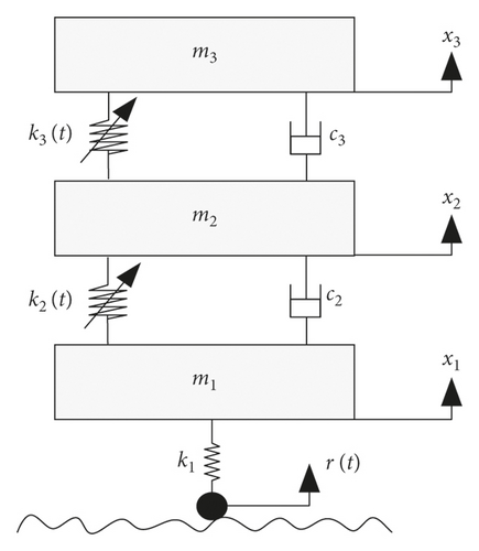
The performance characteristics of the proposed RR-FS-TAR method, along with the LS-FS-TAR method, are examined via Monte Carlo study focused on the identification of a TV three degrees-of-freedom structural system subject to a Gaussian, zero-mean, and uncorrelated excitation r(t), as shown in Figure 1 [3, 30]. Numerical values of the system parameters are given in Table 1.

Details are in the caption following the image — **Figure 1**
Open in figure viewer PowerPoint

Schematic diagram of a TV structural system.

Table 1. Numerical values of the system parameters.

Property	Value
Mass (kg)	m₁ = 0.5, m₂ = 1.5, m₃ = 1.0
Damping (N/(m/s))	c₂ = 0.5, c₃ = 0.3
Stiffness (N/m)	k₁ = 300
	k₂(t) = 100 + 60 sin(2N_sπt/17) + 20 sin(2N_sπt/8.5)
	k₃(t) = 120 + 72 sin(2N_sπt/14.167) + 24 sin(2N_sπt/9.444)

Three cases are considered by choosing different values of the scaling factor N_s. Case 1: slow dynamic evolution with N_s = 0.2, Case 2: medium dynamic evolution with N_s = 1, and Case 3: fast dynamic evolution with N_s = 5. The simulation time is, respectively, 425, 85, and 17 seconds for each case. Given a particular excitation realization, the displacement responses are obtained through the Runge–Kutta 4/5 method characterized by variable integration step and subsequently recorded at a sampling frequency 12 Hz. Therefore, the length of the samples is, respectively, 5100, 1020, and 204 for each case. The above procedure is repeated for each Monte Carlo test (number of tests: 50), with a different excitation realization used each time.

4.1. Case 1: Slow Dynamic Evolution

In this case, the displacement responses are 425s long and the sample length is N = 5100. The AR order is manually selected as n_a = 2 because the actual number of modes present is N_m = 3 and n_a = 2N_m/k = 2, as given by equation (20). The functional basis spanned by trigonometric functions of the form [3, 30],

\begin{matrix} G_{0} [t] = 1, \\ G_{21 i -} [t] = \sin [\frac{i π (t - 1)}{N - 1}], \\ G_{2 i} [t] = \cos [\frac{i π (t - 1)}{N - 1}], i = 1,2, \dots, \end{matrix}

(22)

is selected. The subspace dimensionality p_a = 40 and index b_a = [0 : 39] are selected to approximate the TV model parameters. Figure 2 depicts the LS-based and RR-based natural frequency estimates from the 50 Monte Carlo tests and their true counterparts. As shown in Figure 2 the TV natural frequencies are adequately tracked by the proposed RR-FS-TAR method and the LS-FS-TAR method, due to the relatively larger sample length. However, the proposed RR-FS-TAR method seems to attain better overall performance in terms of tracking and accuracy as the LS-FS-TAR method-based natural frequency estimates exhibit some local tracking errors.

4.2. Case 2: Medium Dynamic Evolution

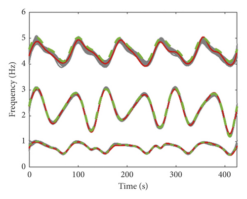
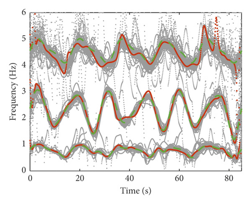
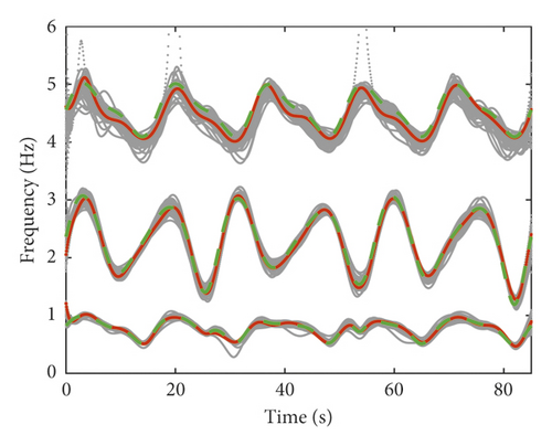
In this case, the displacement responses are 85s long and the sample length is N = 1020. The AR order is selected as n_a = 2. The functional basis spanned by trigonometric functions of equation (22) is here selected with the same values of subspace dimensionality p_a = 40 and index b_a = [0 : 39]. Figure 3 depicts the LS-based and RR-based natural frequency estimates from the 50 Monte Carlo tests and their true counterparts. Evidently, the TV natural frequencies are not adequately tracked by the LS-FS-TAR method and their estimates are quite rough. The trend of the natural frequency estimates obtained by the LS-FS-TAR method is in overall agreement with the true values, but they are of rather poor quality in terms of tracking and accuracy. By contrast, the proposed RR-FS-TAR method attains much better overall performance in terms of tracking and accuracy, even if the system changes faster and the available sample length is relatively shorter.

4.3. Case 3: Fast Dynamic Evolution

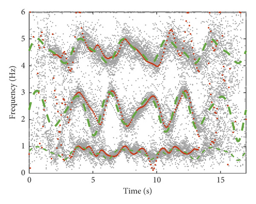
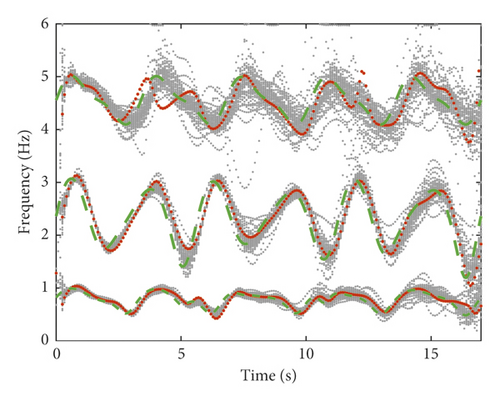
In this case, the system changes appreciably over a relatively short time interval. The displacement responses are 17s long and the sample length is N = 204. The AR order is selected as n_a = 2. The functional basis spanned by trigonometric functions of equation (22) is here selected with the same values of subspace dimensionality p_a = 40 and index b_a = [0 : 39]. Figure 4 depicts the LS-based and RR-based natural frequency estimates from the 50 Monte Carlo tests and their true counterparts. The sample length (N = 204) is much smaller than the number of unknown parameters (k²n_ap_a = 720). In such case, the ordinary least squares estimation is sensitive to errors and may lead to unreliable estimates. This behavior is confirmed by Figure 4, where the TV natural frequencies are not tracked by the LS-FS-TAR method and their estimates are rather vaguely shown or even missing. The proposed RR-FS-TAR method is able to deal with the ill-posed problem via regularization. As shown in Figure 4, the natural frequency estimates obtained by the RR-FS-TAR method is in overall agreement with the true values, although they are rough and exhibit larger tracking errors.

4.4. Power Spectral Density Estimates

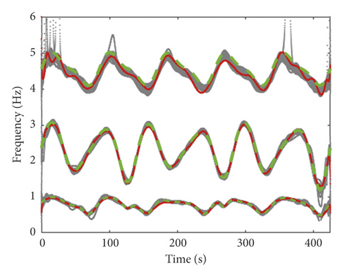
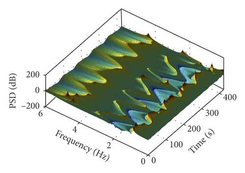
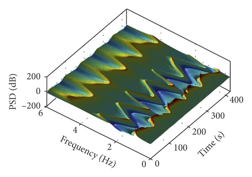
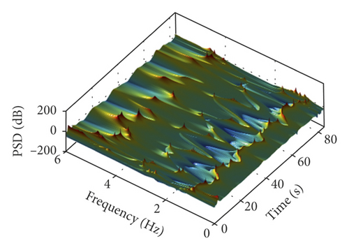
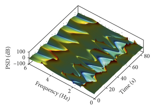
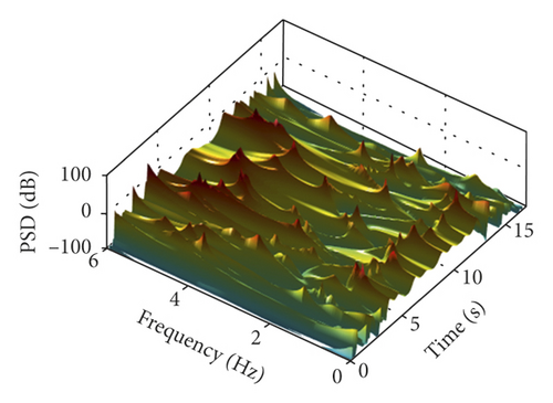
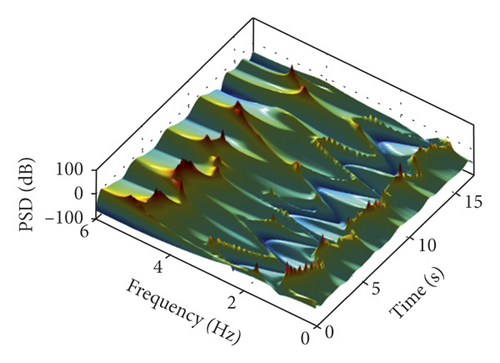
The superior performance of the proposed RR-FS-TAR method is pronounced by the comparison of Figures 2–4 where the estimated natural frequencies are shown. In this section, we further examine the enhanced capability of the RR-FS-TAR method in terms of achievable power spectral density tracking and resolution. Figure 5 depicts the LS-based and RR-based power spectral density estimates from the single test for the TV numerical system with slow, medium, and fast dynamic evolution. The LS-based and RR-based power spectral density estimates are quite similar for the TV numerical system with slow dynamic evolution, as shown in Figure 5. However, with the decrease of the sample length, the LS-FS-TAR method obtains worse results, while the proposed RR-FS-TAR method attains much better performance in terms of tracking and resolution, even if the system changes very fast and the available sample length is quite short (N = 204). In contrast to LS-based FS-TAR estimator requiring larger sample length to represent complicated time-dependencies and dynamics, RR-based FS-TAR estimator is able to track fast dynamic evolution of the system being modeled by using short data.

5. Experimental Validation

5.1. Experimental System

The experimental system [25, 31] is composed of the TV structure, the exciter system (an exciter and a power amplifier), force and motion transducers (an impedance head and 15 accelerometers), the measurement and acquisition module (LMS SCADAS III system), control systems (two Faulhaber DC motors and corresponding motion controllers), and boundary conditions, as shown in Figure 6. The TV structure is a coupled system consisting of a simply supported beam and a moving mass. The mass, driven by two DC motors, can slide on the beam. In this section, two cases are considered by adjusting the moving speed of the mass, as follows: Case 1: the speed is 0.130 m/s and Case 2: the speed is 0.325 m/s.

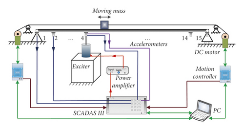
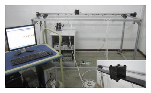
During the test, the mass starts at 0.5 m and stops at 1.8 m. Therefore, the durations for the mass to move over 1.3 m are, respectively, 10 and 4 seconds. The shaker is switched off and removed, and the TV structure is only excited by the motion of the moving mass. Obviously, the interaction between the moving mass and the beam is difficult to measure. Therefore, the excitation of the experimental system is unobservable and the system’s dynamic characteristics have to be determined by exclusively using measured vibration responses. The vibration responses of the simply supported beam are measured by accelerometers, placed at 15 uniformly distributed positions along the beam from left to right, as shown in Figure 6. The acceleration responses are measured at a frequency 512 Hz and subsequently resampled at 256 Hz. Therefore, the length of the samples is, respectively, 2560 and 1024 for the two cases. The above procedure is repeated for each Monte Carlo test (number of tests: 30), and the TV structure undergoes the same variation in each test.

5.2. Identification Results and Discussions

The proposed RR-FS-TAR method and the LS-FS-TAR method are experimentally compared and assessed based on the nonstationary acceleration measurements of the laboratory TV structure. The AR order is manually selected as n_a = 2, and the functional basis spanned by trigonometric functions of equation (22) is selected with the subspace dimensionality p_a = 20 and index b_a = [0 : 19]. Obviously, the sample length (N = 2560 or 1024) is much smaller than the number of unknown parameters (k²n_ap_a = 9000) and the least squares estimation may lead to unreliable estimates.

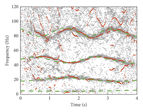
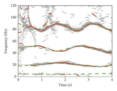
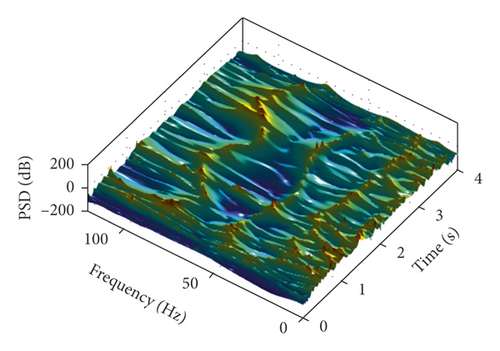
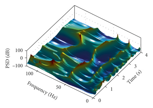
Figure 7 depicts the LS-based and RR-based natural frequency estimates from the 30 Monte Carlo tests when N = 2560. The first four baseline natural frequencies of the TV structure are obtained by using the “frozen-time” technique [31] and denoted by green dashed lines in Figure 7. The gray dots denote the natural frequency estimates from the 30 tests, and the red dots denote the natural frequency estimates from the single test. Evidently, the TV natural frequencies are not adequately tracked by the LS-FS-TAR method and their estimates are quite rough, while the proposed RR-FS-TAR method attains much better tracking performance and the corresponding natural frequency estimates exhibit less false modes. The LS-based and RR-based power spectral density estimates from the single test for the TV structure are also shown in Figure 7. Compared to the LS-based power spectral density estimates, the RR-based estimates appear smoother and are of much better quality in terms of tracking and resolution.

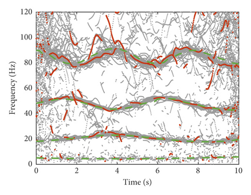
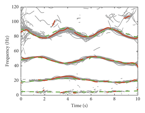
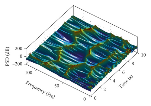
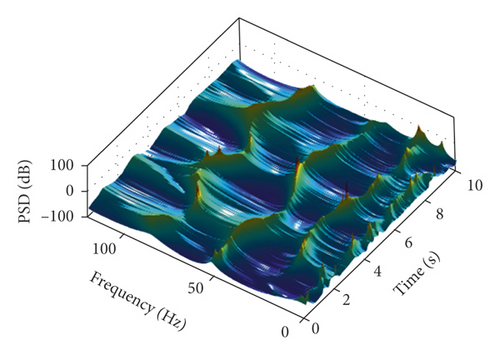
Similarly, Figure 8 depicts the LS-based and RR-based natural frequency estimates from the 30 Monte Carlo tests and power spectral density estimates from the single test when N = 1024. On the one hand, with the decrease of the sample length from 2560 to 1024, both the LS-FS-TAR and RR-FS-TAR methods obtain worse results. Compared to the identification results in Figure 7, natural frequency estimates exhibit larger overall scatter and power spectral density estimates appear more rough, as shown in Figure 8. On the other hand, the enhanced capability of the proposed RR-FS-TAR method is further pronounced to track fast dynamic evolution of the system based on short data. Compared to the LS-based identification results, the RR-based natural frequency estimates exhibit lower overall scatter, less false modes, and smaller tracking errors. Furthermore, the RR-based power spectral density estimates are quite smooth and the ridges are in good agreement with the baseline values, even if the structure changes very fast and the available sample length is relatively short.

For practical systems with larger numbers of degrees-of-freedom and complicated TV dynamics, the number of unknown parameters (k²n_ap_a) of the FS-TAR model is usually quite large. In the meantime, the measured response data length (N) is limited, when systems change appreciably over a relatively short time interval. In such cases, the ordinary least squares estimation may lead to less accurate or even unreliable estimates, and the proposed ridge regression-based FS-TAR method is suggested to identify these systems with fast dynamic evolution based on short data.

6. Conclusions

The FS-TAR model can achieve good representation parsimony, yet it requires a significant number of parameters to represent complicated time-dependencies and dynamics characterized by larger numbers of degrees-of-freedom. Therefore, relatively longer data are usually needed to overcome ill-posed problems and ensure the reliability of least square estimation. However, in many practical cases, systems change appreciably over a relatively short time interval and their dynamics have to be determined based on limited measurement data. In this work, a short data-based output-only identification method for TV systems with fast dynamic evolution was proposed via regularization of ill-posed problems. The proposed ridge regression-based FS-TAR method was employed to identify numerical and experimental systems with different dynamic evolution and compared against the least squares-based FS-TAR method via Monte Carlo study. Comparison results confirm the advantages of the proposed method in terms of achievable natural frequency and power spectral density tracking, accuracy, and resolution of TV systems with fast dynamic evolution, when the available measurement data length is relatively short.

Conflicts of Interest

The authors declare that there are no conflicts of interest.

Acknowledgments

The authors acknowledge the support from the National Natural Science Foundation of China (grant no. 11802201) and China Postdoctoral Science Foundation (grant no. 2017M621075).

Open Research

Data Availability

The data used to support the findings of this study are available from the authors upon request.

References

1 Garibaldi L. and Fassois S., MSSP special issue on the identification of time varying structures and systems, Mechanical Systems and Signal Processing. (2014) 47, no. 1-2, 1–2, https://doi.org/10.1016/j.ymssp.2014.01.010, 2-s2.0-84901192865.
10.1016/j.ymssp.2014.01.010
Web of Science® Google Scholar
2 Niedzwiecki M., Identification of Time-varying Processes, 2000, John Wiley & Sons, New York, NY, USA.
Google Scholar
3 Poulimenos A. G. and Fassois S. D., Parametric time-domain methods for non-stationary random vibration modelling and analysis—a critical survey and comparison, Mechanical Systems and Signal Processing. (2006) 20, no. 4, 763–816, https://doi.org/10.1016/j.ymssp.2005.10.003, 2-s2.0-31044433474.
10.1016/j.ymssp.2005.10.003
Web of Science® Google Scholar
4 Spiridonakos M. D. and Fassois S. D., Non-stationary random vibration modelling and analysis via functional series time-dependent ARMA (FS-TARMA) models—a critical survey, Mechanical Systems and Signal Processing. (2014) 47, no. 1-2, 175–224, https://doi.org/10.1016/j.ymssp.2013.06.024, 2-s2.0-84901194728.
10.1016/j.ymssp.2013.06.024
Web of Science® Google Scholar
5 Rao T. S., The fitting of non-stationary time-series models with time-dependent parameters, Journal of the Royal Statistical Society: Series B (Methodological). (1970) 32, no. 2, 312–322, https://doi.org/10.1111/j.2517-6161.1970.tb00844.x.
10.1111/j.2517-6161.1970.tb00844.x
Web of Science® Google Scholar
6 Mendel J. M., Discrete Techniques of Parameter Estimation: The Equation Error Formulation, 1973, Marcel Dekker, New York, NY, USA.
Google Scholar
7 Kozin F., Estimation and modeling of nonstationary time series, Proceedings of the Symposium of Applications of Computer Mathod in Engineering, August 1977, Los Angeles, CA, USA, 603–612.
Google Scholar
8 Grenier Y., Time-dependent ARMA modeling of nonstationary signals, IEEE Transactions on Acoustics, Speech, and Signal Processing. (1983) 31, no. 4, 899–911, https://doi.org/10.1109/tassp.1983.1164152, 2-s2.0-0020798029.
10.1109/TASSP.1983.1164152
Web of Science® Google Scholar
9 Grenier Y., Estimation of non-stationary moving average models, Proceedings of the IEEE International Conference on Acoustics, Speech, and Signal Processing (ICASSP ‘83), April 1983, Boston, MA, USA, 268–271.
Google Scholar
10 Grenier Y., Time-frequency analysis using time-dependent ARMA models, Proceedings of the IEEE International Conference on Acoustics, Speech, and Signal Processing (ICASSP ‘84), January 1984, San Diego, CA, USA, 270–273.
Google Scholar
11 Chevalier M., Chollet C., and Grenier Y., Speech analysis and restitution using time-dependent autoregressive models, Proceedings of the IEEE International Conference on Acoustics, Speech, and Signal Processing (ICASSP ‘85), 1985, Tampa, FL, USA, 501–504.
Google Scholar
12 Grenier Y., Nonstationary ARMA models via simultaneous AR and MA estimation, Proceedings of the IEEE International Conference on Acoustics, Speech, and Signal Processing (ICASSP ‘86), 1986, Tokyo, Japan, 2339–2342.
Google Scholar
13 Gersh W. and Kitagawa G., A time-varying multivariate autoregressive modeling of econometric time series, Proceedings of the Business and Statics ASA Annual Meeting, 1983, Toronto, Canada, 399–404.
Google Scholar
14 Niedzwiecki M., Functional series modeling approach to identification of nonstationary stochastic systems, IEEE Transactions on Automatic Control. (1988) 33, no. 10, 955–961, https://doi.org/10.1109/9.7254, 2-s2.0-0024089490.
10.1109/9.7254
Web of Science® Google Scholar
15 Niedzwiecki M., Recursive functional series modeling estimators for identification of time-varying plants-more bad news than good?, IEEE Transactions on Automatic Control. (1990) 35, no. 5, 610–616, https://doi.org/10.1109/9.53509, 2-s2.0-0025432207.
10.1109/9.53509
Web of Science® Google Scholar
16 Tsatsanis M. K. and Giannakis G. B., Time-varying system identification and model validation using wavelets, IEEE Transactions on Signal Processing. (1993) 41, no. 12, 3512–3523, https://doi.org/10.1109/78.258089, 2-s2.0-0027807710.
10.1109/78.258089
Web of Science® Google Scholar
17 Tsatsanis M. K. and Giannakis G. B., Modelling and equalization of rapidly fading channels, International Journal of Adaptive Control and Signal Processing. (1996) 10, no. 23, 159–176, https://doi.org/10.1002/(sici)1099-1115(199603)10:2/3<159::aid-acs346>3.3.co;2-d.
10.1002/(SICI)1099-1115(199603)10:2/3<159::AID-ACS346>3.0.CO;2-M
Web of Science® Google Scholar
18 Spiridonakos M. D. and Fassois S. D., Parametric identification of a time-varying structure based on vector vibration response measurements, Mechanical Systems and Signal Processing. (2009) 23, no. 6, 2029–2048, https://doi.org/10.1016/j.ymssp.2008.11.004, 2-s2.0-67349244887.
10.1016/j.ymssp.2008.11.004
Web of Science® Google Scholar
19 Spiridonakos M. D. and Fassois S. D., Adaptable functional series TARMA models for non-stationary signal representation and their application to mechanical random vibration modeling, Signal Processing. (2014) 96, 63–79, https://doi.org/10.1016/j.sigpro.2013.05.012, 2-s2.0-84887413191.
10.1016/j.sigpro.2013.05.012
Web of Science® Google Scholar
20 Yang W., Liu L., Zhou S.-D., and Ma Z.-S., Moving kriging shape function modeling of vector TARMA models for modal identification of linear time-varying structural systems, Journal of Sound and Vibration. (2015) 354, 254–277, https://doi.org/10.1016/j.jsv.2015.06.004, 2-s2.0-84955642317.
10.1016/j.jsv.2015.06.004
Web of Science® Google Scholar
21 Zhou S.-D., Ma Y.-C., Liu L., Kang J., Ma Z.-S., and Yu L., Output-only modal parameter estimator of linear time-varying structural systems based on vector TAR model and least squares support vector machine, Mechanical Systems and Signal Processing. (2018) 98, 722–755, https://doi.org/10.1016/j.ymssp.2017.05.026, 2-s2.0-85022219328.
10.1016/j.ymssp.2017.05.026
Web of Science® Google Scholar
22 Bertha M. and Golinval J.-C., Identification of non-stationary dynamical systems using multivariate ARMA models, Mechanical Systems and Signal Processing. (2017) 88, 166–179, https://doi.org/10.1016/j.ymssp.2016.11.024, 2-s2.0-85008263108.
10.1016/j.ymssp.2016.11.024
Web of Science® Google Scholar
23 Li W., Vu V.-H., Liu Z., Thomas M., and Hazel B., Application of adaptable functional series vector time-dependent autoregressive model for extraction of real modal parameters for identification of time-varying systems, Measurement. (2017) 103, 143–156, https://doi.org/10.1016/j.measurement.2017.02.027, 2-s2.0-85014100182.
10.1016/j.measurement.2017.02.027
Web of Science® Google Scholar
24 Ma Z.-S., Liu L., Zhou S.-D., and Yu L., Output-only modal parameter recursive estimation of time-varying structures via a kernel ridge regression FS-TARMA approach, Shock and Vibration. (2017) 2017, 14, 8176593, https://doi.org/10.1155/2017/8176593, 2-s2.0-85010670203.
10.1155/2017/8176593
Web of Science® Google Scholar
25 Ma Z.-S., Liu L., Zhou S.-D. et al., Parametric output-only identification of time-varying structures using a kernel recursive extended least squares TARMA approach, Mechanical Systems and Signal Processing. (2018) 98, 684–701, https://doi.org/10.1016/j.ymssp.2017.05.013, 2-s2.0-85022229382.
10.1016/j.ymssp.2017.05.013
Web of Science® Google Scholar
26 Walter G. G., Wavelets and Other Orthogonal Systems with Applications, 1994, Taylor & Francis, Boca Raton, FL, USA.
Google Scholar
27 Lütkepohl H., Handbook of Matrices, 1996, John Wiley & Sons, New York, NY, USA.
Google Scholar
28 Tikhonov A. N., Goncharsky A. V., Stepanov V. V., and Yagola A. G., Numerical Methods for the Solution of Ill-Posed Problems, 1995, Springer Science & Business Media, Dordrecht, Netherlands.
10.1007/978-94-015-8480-7
Google Scholar
29 Hoerl A. E. and Kennard R. W., Ridge regression: biased estimation for nonorthogonal problems, Technometrics. (1970) 12, no. 1, 55–67, https://doi.org/10.1080/00401706.1970.10488634, 2-s2.0-84942484786.
10.1080/00401706.1970.10488634
Web of Science® Google Scholar
30 Poulimenos A., Spiridonakos M., and Fassois S., Parametric time-domain methods for non-stationary random vibration identification and analysis: an overview and comparison, Proceedings of the ISMA2006 International Conference on Noise and Vibration Engineering, September 2006, Leuven, Belgium, 2885–2905.
Google Scholar
31 Ma Z.-S., Liu L., Zhou S.-D., and Yang W., Modal parameter estimation of the coupled moving-mass and beam time-varying system, Proceedings of the ISMA2014 International Conference on Noise and Vibration Engineering, 2014, Leuven, Belgium, 587–596.
Google Scholar

Citing Literature

All articles

Short Data-Based Output-Only Identification for Time-Varying Systems with Fast Dynamic Evolution

Abstract

1. Introduction