1. Introduction

An automobile engine is a core component of a car powered by fuel, and its structure is complicated. The failure of a part not only affects the machine operation but may also cause considerable economic losses or even catastrophic consequences. Common engine failures include wear, distortion, cavitation, and corrosion, and different faults can be detected in various approaches, such as tail gas, power and speed, oil, and vibration and noise analytical methods [1–5].

In comparison with other detection methods, the use of acoustic signals for extracting fault components has the advantage of detection without disassembling devices. The abnormal noise and vibration signals of an engine often contain considerable dynamic information about the engine state, including fault components, acoustic signals of other components working properly, and background noise [6]. The fault component of some faults often has quasi-periodicity. By processing abnormal sound signals, the extracted fault component can be used as an effective basis for analysing the cause of engine fault. As the fault component of abnormal signals has a low signal-to-noise ratio, the extraction of fault components is often the most important and difficult problem, which directly affects the accuracy and reliability of diagnosis [7]. Methods for processing abnormal noise signals mainly include fast Fourier transform (FFT), wavelet transform, and empirical mode decomposition (EMD) [5, 8, 9]. Classical signal processing methods, such as FFT and short-time Fourier transform, cannot analyse strong nonlinear and nonstationary signals. Wavelet analysis can have good localization characteristics in the time and frequency domains; thus, it is often used to extract time-frequency characteristics [10]. Figlus [11] used a continuous wavelet transform (CWT) to process vibration signals qualitatively, and they quantitatively identified the damage degree of the timing chain tensioner. Figlus [5, 12] used the discrete wavelet transform (DWT) and wavelet packet decomposition to detect the valve clearance of a diesel engine automatically. Albarbar [13] proved that CWT is sensitive to the engine speed and load change by using it to manage diesel engine acoustic signals. Shirazi and Mahjoob [14] used the DWT transfer vibration signals of a typical four-cylinder engine from the time domain to the time-frequency domain for fault detection. Although the wavelet transform has the advantage of multiresolution analysis of signals, appropriate wavelet basis functions are difficult to be selected before processing signals [15]. To solve this problem, Huang et al. [9] proposed the EMD, which can efficiently decompose nonlinear and nonstationary signals without any set of basis functions. Vernekar et al. [16] presented an engine gearbox fault diagnosis on the basis of EMD and naive Bayes algorithm to manage vibration signals. They classified healthy and different simulated faulty conditions of gear and bearing, and results showed that the classification accuracy of their method can reach 98.88%. Zhao et al. [17] combined the EMD and autoregressive model to diagnose the faults of crankshaft bearing and connecting rod bearing and obtained the fault spectrum. To overcome the noise effects, Xu et al. [18] proposed a new method for engine vibration diagnosis on the basis of an EMD adaptive threshold filter and presented the correlation dimension. Experimental results indicated that the proposed method can effectively remove the noise of engine vibration signal and improve the accuracy and efficiency of EMD. Ye and Shao [19] introduced a new inspection method based on EMD and envelope spectrum analysis to analyse vibration signals. Results showed that the proposed method has excellent performance in quality inspection in the presence of abnormal clearance between the engine crankshaft and connecting rod. Tan et al. [20] used the EMD method to remove diesel engine vibration signals. Test results indicated that the true vibration signal from the diesel engine could be obtained by reconstructing the remaining IMF components. Although EMD has been successfully applied in the field of fault diagnosis, it has limitations, such as the frequent occurrence of mode mixing. To overcome this problem, Wu and Huang [21] proposed ensemble empirical mode decomposition (EEMD) in 2009. EEMD adds finite amplitude Gauss white noise to the signal when the signal is decomposed, thereby eliminating mode mixing to a certain extent. Wang et al. [6] presented a new adaptive wavelet packet thresholding function based on adaptive wavelet threshold denoising, EEMD, and correlation dimension for vibration signal denoising. This new method can effectively extract the impact signal features induced by vibrations. Zhang et al. [22] used EEMD and other methods to process engine abnormal sound and the frequency-dependent contributions of different engine parts to different test points under different speeds.

In recent years, numerous scientists have proposed processing methods for nonstationary signals. Smith [23] introduced the local mean decomposition (LMD) method in 2005. Frei and Osorio [24] presented the intrinsic time-scale decomposition (ITD) method in 2007. However, similar to the EMD, the LMD and ITD have the disadvantage of mode mixing. In 2015, Dayong et al. [25] proposed a dislocation superimposed method (DSM) on the basis of the random decrement technique. In comparison with other methods, the DSM is simple and will not change the concerned component in the mixed signal. The fault component is a quasi-periodic signal; thus, it requires people to select the starting point and superposition length when DSM is used to process abnormal acoustic signals, which greatly reduce the efficiency of processing experimental data. This paper presents a developed DSM for automatically extracting the impulsive fault component from the abnormal noise signal of an engine.

2. DSM Review

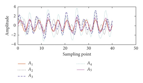
Figure 1 presents a simple example of the DSM, where A₁ and A₂ are two periodic signals with different periods and amplitudes, in which A₁ indicates the target signal and its period is T. A₃ refers to a synthetic signal of A₁ and A₂. To extract A₁ from the mixed signal A₃, A₃ is moved to the right for T and then added with A₃ to obtain A₄. The period of A₁ does not change, but the amplitude is doubled during superposition, whereas A₂ is destroyed. Repeating the previous process can increase the amplitude of the target signal. Dividing the superimposed signal by the corresponding superposition number can obtain the target signal.

3. Introduction of Improved DSM

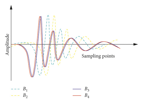
A slight change in the engine speed is observed. Thus, the impulsive fault components generated by certain parts are quasi-periodic signals, as shown in Figure 2, which could not be extracted by moving the fault component cycle. Therefore, artificially selecting a suitable starting point is necessary at the front end of each dislocation superimposed interception signal containing fault components. To overcome the shortcomings of human participation in processing data, this paper presents a developed DSM for automatically extracting impulsive fault components from the abnormal noise signal of an engine. This new method consists of three steps: selection of starting points, superimposition of interception signal, and separation of fault components.

3.1. Selection of the Starting Points of Dislocation Superimposed Interception Signal

Ideal starting points represent the first point of each fault component. However, the position of fault components is difficult to determine due to the nonstationary feature of abnormal sound signals. Thus, a suitable point in the vicinity of the position where the fault component exists must be selected as the starting point.

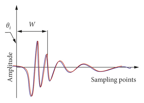
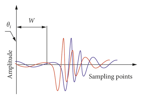
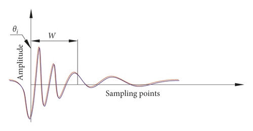
Assume that the engine produces an impulsive fault every q revolutions of the crankshaft. The angle of q revolutions is divided into H parts. Then, an area of length w (W area) is intercepted at any phase, where w represents the length of the initial area containing the main energy of the fault component. Waveforms of the W area in abnormal sound at different times are similar. Therefore, W₁ and W₂ are intercepted at the same phase of two consecutive q revolutions for correlation analysis. ρ(W₁, W₂) and M₁ (which is a threshold for preliminarily judging whether the phase position can be used as the starting point) are compared. If the W₁ and W₂ areas include the main energy area of two fault components, as shown in Figure 3(a), where ρ(W₁, W₂) is greater than M₁, then the starting point is preliminarily selected at the phase. If the W₁ and W₂ areas contain background noise or few fault components, as shown in Figure 3(b), where ρ(W₁, W₂) is less than M₁, then the starting point should be reverified at the next phase.

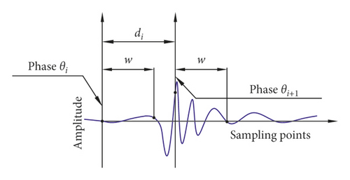
A positional deviation may exist between the fault components intercepted at the same phase of different revolutions due to slight changes in the engine speed during operation. Figure 4 shows that ρ(W₁, W₂) calculated at θ_i is greater than M₁; however, a large positional deviation is observed between the fault components. The fault component will be destroyed in the superimposition process. Therefore, the starting point could not be selected at phase θ_i and must be reverified at θ_i+1. When the phase is constantly approaching the position where the fault component exists, the positional deviation between the fault components is gradually reduced. If the deviation can be regarded as a natural error, then the starting point can be determined at the phase.

To determine whether the positional deviation between the fault features is negligible, some W areas are superimposed, and the correlation coefficient between the superimposed W areas is calculated under the same number of superposition times. If the correlation increases with the number of superpositions, then the positional deviation can be ignored. The steps of the judgment method are as follows:

Step 1. Divide consecutive 2m W areas at the same phase of different revolutions into two groups in accordance with the parity of serial numbers and guarantee that samples 2m are enough. Superimpose W areas in each group by using the following equation:

$$\begin{array}{}{D}_{Wuk}=\frac{1}{k+1}\sum _{j=1}^{k+1}{W}_{22j+u-},\end{array}$$ (3)

where D_Wuk is the superimposed W areas; u denotes the group number, u = 1, 2; and k indicates the number of superpositions, k = 1, 2, 3, …, m − 1.

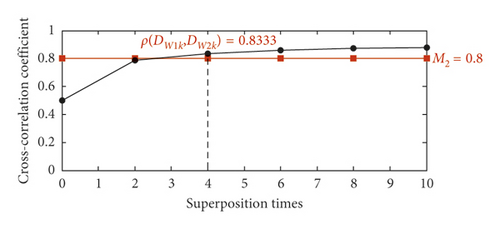
Step 2. Calculate the correlation coefficient ρ(D_W1k, D_W2k) between superimposed signals D_W1k and D_W2k under the same number of superpositions, as shown in Figure 5. If ρ(D_W1k, D_W2k) increases with the number of superpositions until it is greater than threshold M₂ (M₂ is for assessing whether the positional deviation is negligible), then the positional deviation can be ignored, and the selected starting point is valid. Otherwise, the starting point is preliminarily assessed again at the next phase.

ρ(D_W1k, D_W2k) is not strictly monotonous with the number of superpositions due to the influence of background noise. Hence, ρ(D_W1k, D_W2k) is indirectly compared under the number of superpositions by using the following equation:

$$\begin{array}{}\rho \left(D_{W1\left(k+2\right)},D_{W2\left(k+2\right)}\right)>\rho \left(D_{W1k},D_{W2k}\right).\end{array}$$ (4)

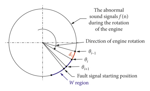
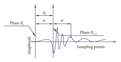
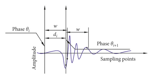
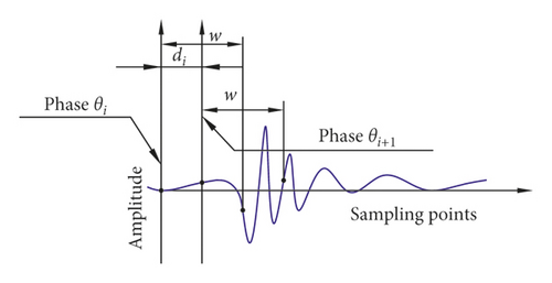
A phenomenon that the fault component is destroyed when ρ(W₁, W₂) is greater than M₁ also exists, as shown in Figure 6. To solve this problem, H parts of the angle of q revolutions must be sufficient to satisfy d_i < w/2, where d_i is the length of the abnormal signal between phases θ_i and θ_i+1. The reason is that ρ(W₁, W₂) must be recalculated at phase θ_i+1 and compared with M₁ when ρ(W₁, W₂) at phase θ_i is less than M₁. If d_i ≥ w, then the main energy area of the fault components will be destroyed or skipped, as shown in Figures 7(a) and 7(b). If w/2 ≤ d_i < w, then the main energy area is destroyed, as shown in Figure 7(c). If d_i < w/2, then the main energy area is hardly destroyed. In this study, d_i < w/5.

In addition, if the first ρ(W₁, W₂) is greater than M₁, then the result is discarded and ρ(W₁, W₂) is recalculated at the next phase until it is less than M₁ and then greater than M₁ again.

Considering the different lengths of the main energy areas of different fault characteristics, w should be set to a fixed value to select the valid starting point when different types of faults occur. This study obtains the value of w using equation (5) by studying numerous impulsive signals and referring to the length of the main energy area of fault signals in other studies, as shown in Table 1. The length of the main energy area is determined through experience:

$$\begin{array}{}w=\frac{h}{44100}\times 300.\end{array}$$ (5)

Equation (5) is an empirical formula, which can effectively separate impulsive fault components, including cylinder knocking and connecting rod bearing knocking; however, its versatility needs further verification.

When slight changes in engine speed are not considered, d_i is calculated using the following equation:

$$\begin{array}{}{d}_i=\frac{60qh}{\omega H},\end{array}$$ (6)

where d_i is the length of the abnormal signal between phases θ_i and θ_i+1, q denotes the number of revolutions of the crankshaft, h represents the sampling frequency, ω indicates the engine rotating speed, and H refers to the number of parts into which the angle of q revolutions is divided.

Therefore, H should satisfy the following equation:

$$\begin{array}{}H\ge \frac{300qh}{w\omega }.\end{array}$$ (7)

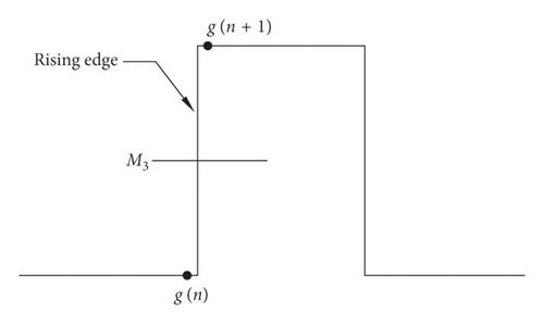
The encoder can generate a certain number of pulse signals, and the angle between any adjacent pulse signals is equal. The encoder is used to divide the angle in the experiment. Figure 8 and equation (8) show that M₃ is a threshold for assessing the rising edge of the pulse signal. Two consecutive discrete points g(n) and g(n + 1) of the pulse signal are compared with threshold M₃. When g(n) is smaller and g(n + 1) is larger than M₃, a rising edge is considered to exist between points:

$$\begin{array}{}g\left(n\right)<M_3<g\left(n+1\right).\end{array}$$ (8)

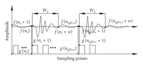
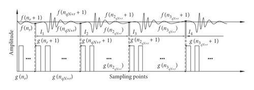
The W areas are obtained as follows: simultaneous data acquisition of the abnormal sound signal f(n) and pulse signal g(n) is conducted under the same sampling frequency and one-to-one correspondence between signal data points. In Figure 9 and equation (9), f(n_r + 1) corresponding to g(n_r + 1) is selected as the starting point, and w points are intercepted backward as W areas:

$$\begin{array}{}{W}_j=f\left(n_{\left(j-1\right)qN+r}+123,n_{\left(j-1\right)qN+r}+,n_{\left(j-1\right)qN+r}+,\dots ,n_{\left(j-1\right)qN+r}+w\right),\end{array}$$ (9)

where j is the serial number of the W areas, j = 1, 2, 3, …; r denotes the serial number of the rising edge, r = 1, 2, 3, …; q represents the number of revolutions of the crankshaft; and N indicates the number of pulses triggered by the encoder at one revolution.

Table 1. Length of the main energy areas of engine fault components and mechanical faults found in other studies.

Serial number	Failure type	Sampling rate	Main peak area length
1	Fuel injection advance angle fault [6]	48 kHz	Approximately 180
2	Enlarged clearance case for cylinder intake valve and exhaust valve [12]	25.6 kHz	Approximately 45
3	Cylinder misfire fault [25]	44.1 kHz	Approximately 150
4	Abraded connecting rod bearing shell faults [25]	44.1 kHz	Approximately 150
5	Bolt loosening faults [25]	44.1 kHz	Approximately 100
6	Roller bearing with outer race fault [26]	12 kHz	Approximately 40
7	Bearing with inner race defect [27]	12 kHz	Approximately 40
8	Piston slap noise [28]	25.6 kHz	Approximately 120
9	Combustion chamber knock [29]	100 kHz	Approximately 200
10	Wear of crankshaft bearing [30]	12.8 kHz	Approximately 70

3.2. Superposition of Abnormal Sound Signals

The abnormal sound signal is divided into different segments I_j at valid phases. Different sections I_j are superimposed to improve the signal-to-noise ratio.

I_j is obtained as follows: in Figure 10 and equation (10), f(n_(j−1)qN+r + 1) corresponding to g(n_(j−1)qN+r + 1), which is used to assess the ((j − 1)qN + r)th rising edge, is selected as the first point of I_j, and f(n_jqN+r) corresponding to g(n_jqN+r), which is used to judge the (jqN + r)th rising edge, is set as the last point of I_j:

$$\begin{array}{}{I}_j=f\left(n_{\left(j-1\right)qN+r}+123,n_{\left(j-1\right)qN+r}+,n_{\left(j-1\right)qN+r}+,\dots ,n_{jqN+r}\right),\end{array}$$ (10)

where j is the serial number of the I_j areas, j = 1, 2, 3, …; r denotes the serial number of the rising edge, r = 1, 2, 3, …; q represents the number of revolutions of the crankshaft; and N indicates the number of pulses triggered by using the encoder at one revolution.

Superimposition is conducted as follows: consecutive 2m segments I_j are divided into two groups in accordance with the parity of serial numbers. W areas are superimposed using equation (11) in each group. The superimposed length is the minimum length of 2m segments:

$$\begin{array}{}{D}_{Iuk}=\frac{1}{k+1}\sum _{j=1}^{k+1}{I}_{22j+u-},\end{array}$$ (11)

where D_Iuk is the superimposed segment signals; u indicates the group number, u = 1, 2; and k denotes the number of superpositions when ρ(D_W1k, D_W2k) is greater than M₂.

3.3. Separation of Fault Components

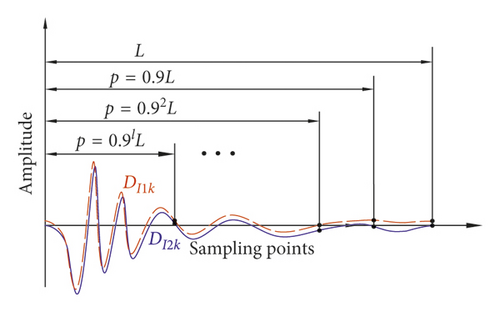
The superimposed segments are composed of the noise-reduced fault component and superimposed background noise. The fault component is located at the front end of the superimposed segment signal. Therefore, the superimposed segments must be divided to separate the fault features.

Figures 11(a) and 11(b) show the separation method. The correlation coefficient ρ(P_1k(l), P_2k(l)) between the areas of length p (P areas) of the front end of the superimposed segments D_Iuk is calculated. ρ(P_1k(l), P_2k(l)) is compared with M₄ (which is the threshold for assessing fault characteristics). If ρ(P_1k(l), P_2k(l)) is greater than threshold M₄, then the P area can be regarded as a fault component. If ρ(P_1k(l), P_2k(l)) is smaller than M₄, then the length of the P area is modified to 90% of the original length and then rounded down. ρ(P_1k(l), P_2k(l)) is recalculated and compared with M₄. The selection of starting point is a process of fixed length analysis that fails to determine the amount of fault components in the W area. The fault component can be qualitatively separated by comparing ρ(P_1k(l), P_2k(l)) with M₄. M₄ should be smaller than ρ(D_W1k, D_W2k) to ensure that the length of the separated fault component is greater than w. In this study, M₄ is set to ρ(D_W1k, D_W2k)−0.05, and the initial value of p is set to 0.9 × L, where L is the length of the superimposed segments. The P area is calculated using the following equations:

$$\begin{array}{}{P}_{uk}\left(l\right)=D_{Iuk}\times R_2\left(n\right),\end{array}$$ (12)

$$\begin{array}{}{R}_2\left(n\right)=10,\le n\le ⌊{0.9}^l\times L⌋,\end{array}$$ (13)

where P_uk(l) is the area of length p of the front end of the superimposed segments D_Iuk; R₂(n) represents a rectangular window function with a length of 0.9^l × L; l denotes the number of times that the length of the P area changes, l = 1, 2, 3, …; u indicates the group number, u = 1, 2; k is the number of superpositions when ρ(D_W1k, D_W2k) is greater than M₂; and L refers to the length of the superimposed segments. ⌊.⌋ is a round-down function.

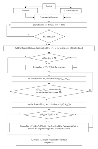
The developed DSM encompasses all of the above steps, and the flow chart of Figure 12 is drawn for a better understanding of the method.

4. Experiment Condition

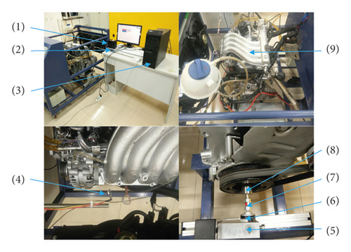
Figure 13 shows the physical diagrams of the experimental bench. The data acquisition system consists of acoustic sensors, encoders, data acquisition cards, and computers. The acoustic sensor with a frequency ranging from 20 Hz to 20 kHz is placed above the cylinder to receive the abnormal sound signals generated by the engine. The encoder model is ZSP3806GC, which triggers 100 electrical pulses per revolution. The encoder can synchronously revolve with the crankshaft by fixing it on the front end of the crankshaft through a coupling. The data acquisition card model is USB-6341 produced by the National Instruments Company. The sampling frequency is 44100 Hz. Data acquisition and processing are conducted using MATLAB software. The engine of the experimental stand was disassembled from a car, whose parameters are shown in Table 2.

5. Experimental Data Processing

Figure 14 presents the abnormal signal caused by the fault of cylinder knocking and pulse signal triggered by the encoder under high speed (1800 r/min). We can observe the considerable difference from the normal and faulty acoustic signals.

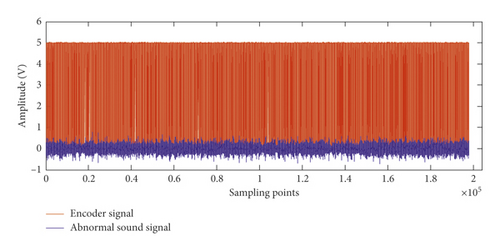
The improved DSM is used to process the abnormal sound signal. Firstly, the angle of the two revolutions of the crankshaft is divided into 100 parts, that is, dividing 200 rising edges into 100 parts, which satisfies the requirements of equation (7) (H should be greater than 49), to ensure that each intercepted segment contains a fault component. Threshold M₁ is set to 0.3. Secondly, ρ(W₁, W₂) is calculated at different rising edges. Table 3 shows the ρ(W₁, W₂) values calculated from the first to the ninth rising edges. ρ(W₁, W₂) calculated at the ninth rising edge is 0.5012, which is greater than M₁. Therefore, the starting point is preliminarily selected at the position of the rising edge. Thirdly, the 22 W areas acquired at the ninth rising edge are divided into two groups. The odd- and even-numbered W areas are the first and second groups, respectively. Threshold M₂ is set to 0.8. Figure 15 shows ρ(D_W1k, D_W2k) under different superposition numbers (ρ(D_W10, D_W20) represents ρ(W₁, W₂)). ρ(D_W14, D_W24) is greater than M₂, and ρ(D_W1k, D_W2k) increases with the number of superpositions under the superimposing condition of 1–4 times. Hence, the starting point selected at the ninth rising edge is valid.

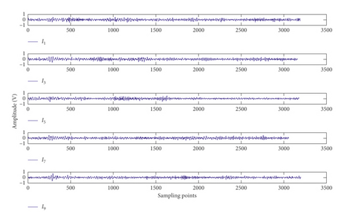
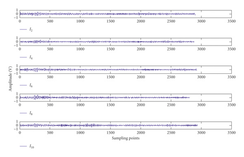
Equation (10) is used to intercept the abnormal signal per two revolutions of the crankshaft at the ninth rising edge. Ten intercepted sections are divided into two groups on the basis of the parity of serial numbers, and Figures 16(a) and 16(b) show the sections. Then, the intercepted sections are superimposed four times in each group; the superimposed length is 2739. Figure 17 presents the result.

Finally, in order to separate fault components, the initial value of p is set to ⌊0.9 × 2739⌋ = 2465 and threshold M₄ is set to ρ(D_W14, D_W24) − 0.05 = 0.7833. The correlation coefficient between the P areas of two superimposed signals is calculated. ρ(P₁₄(15), P₂₄(15)) is 0.7860 after p changed 15 times, which is greater than M₄. Thus, P_u4(15) can be regarded as fault components, as shown in Figure 18. Although the front end of the isolated faulty component contains a minimal background noise, most of the noise has been removed.

The result proves that the developed DSM can automatically extract the fault features from the abnormal sound. If traditional DSM is used in this chapter, we need to slowly select the appropriate starting point, which greatly reduces the computational efficiency.

6. Other Applications of the Developed Method

To verify the applicability of the developed method, the abnormal noise signal of the connecting rod bearing knocking is collected under a speed of 1100 r/min, as shown in Figure 19. Data acquisition and processing methods are the same as before, and the sampling rate is 44100 Hz.

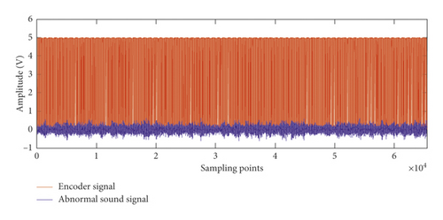
The angle of one revolution of the crankshaft is divided into 100 parts, which satisfies the requirements of equation (7) (H should be greater than 45). Threshold M₁ is set to 0.3. Table 4 shows ρ(W₁, W₂) calculated from the first to the 23rd rising edges, and ρ(W₁, W₂) calculated at the 23rd rising edge is greater than M₁. Hence, the starting point is preliminarily selected at the position of the 23rd rising edge.

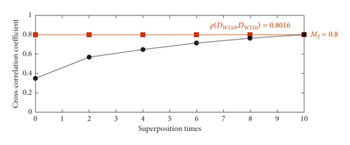
Figure 20 shows ρ(D_W1k, D_W2k) under 1–10 numbers of superposition. Threshold M₂ is set to 0.8. ρ(D_W110, D_W210) is 0.8016, which is greater than M₂, and ρ(D_W1k, D_W2k) increases with the number of superpositions under the superimposing condition of 1–10 times. Thus, the starting point selected at the 23rd rising edge is valid.

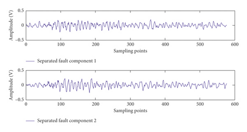
The abnormal signal per revolution of the crankshaft is intercepted at the 23rd rising edge. The 22 intercepted sections are divided into two groups and superimposed. Figure 21 shows the result. The initial value of p is ⌊0.9 × 2522⌋ = 2269, and threshold M₄ is ρ(D_W14, D_W24) − 0.05 = 0.7516. ρ(P₁₁₀(14), P₂₁₀(14)) is greater than M₄ after changing 14 times. Thus, P_u10(14) can be regarded as fault components, as shown in Figure 22.

From the above two examples, we find that the improved method can automatically extract the component of impulsive signal from the abnormal noise signal of an engine. However, the new method is currently only effective at a single speed range and cannot process signals at different speed range. The reason is that the same sampling rate and varying speed result in a large difference in length between different fault features in W regions so that the correct starting point cannot be selected.

7. Precision Analysis

Damaged parts are artificially used to create a fault component, which is regarded as an actual fault component, with high signal-to-noise ratio in a quiet environment. The separated fault component is compared with the actual fault component for accuracy analysis. Figure 23 shows the areas of remarkable characteristics with a length of 300 of the actual and separated fault components of cylinder knocking. This area is used for analysis to avoid interference from background noise at the rear end of the artificially manufactured fault component. Separated fault components 1 and 2 are the segments of P₁₄(15) and P₂₄(15), respectively. The correlation coefficient between separated fault components 1 and 2 and the actual fault component are 0.7346 and 0.6655, respectively. Figure 24 presents the actual and separated fault components of connecting rod bearing knocking after normalization. The correlation coefficient between separated fault components 1 and 2 and the actual fault component are 0.8452 and 0.8685, respectively.

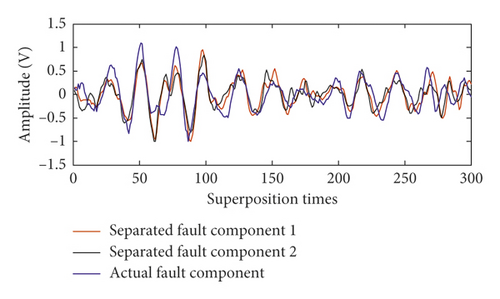
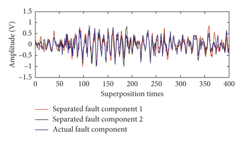
On the basis of the analysis result, the developed method can effectively extract fault characteristics from an abnormal sound signal, and we can change the value of M₂ to increase the number of superimpositions for improving the accuracy of separated fault components.

To classify the damage, a database contained different fault characteristics should be built. The fault waveform is separated from complex noise by the developed DSM when engine fails. Next, the fault types can be determined by comparing the separated fault features with those in the database or classification methods such as neural networks.

8. Conclusion

In this study, a developed DSM is used to extract the characteristics of cylinder knocking and connecting rod bearing knocking automatically from the abnormal sound signal of the engine. The main conclusions are as follows.

The traditional DSM is a theoretical algorithm for ideal uniform velocity conditions, and it cannot analyse actual abnormal noise signals independently. The developed method can automatically select appropriate starting points to superimpose the abnormal sound signals and finally separate the fault characteristics. Although the front end of the separated fault component contains minimal noise, most of the noise has been removed. Generally, the new method greatly improves the practicability, has a good application prospect, and supplements the methods of extracting fault features in the time domain.

Conflicts of Interest

The authors declare that there are no conflicts of interest regarding the publication of this paper.