International Journal of Differential Equations

Volume 2019, Issue 1 7609879

Research Article

Open Access

Advanced Analytical Treatment of Fractional Logistic Equations Based on Residual Error Functions

Saleh Alshammari

orcid.org/0000-0001-9604-1680

Centre for Modelling and Data Science, Faculty of Science and Technology, Universiti Kebangsaan Malaysia, 43600 Bangi, Selangor, Malaysia ukm.my

Search for more papers by this author

Mohammed Al-Smadi,

Corresponding Author

Mohammed Al-Smadi

[email protected]

orcid.org/0000-0003-0226-7254

Department of Applied Science, Ajloun College, Al-Balqa Applied University, Ajloun 26816, Jordan bau.edu.jo

Search for more papers by this author

Mohammad Al Shammari,

Mohammad Al Shammari

Centre for Modelling and Data Science, Faculty of Science and Technology, Universiti Kebangsaan Malaysia, 43600 Bangi, Selangor, Malaysia ukm.my

Search for more papers by this author

Ishak Hashim,

Ishak Hashim

orcid.org/0000-0003-4237-7140

Centre for Modelling and Data Science, Faculty of Science and Technology, Universiti Kebangsaan Malaysia, 43600 Bangi, Selangor, Malaysia ukm.my

Search for more papers by this author

Mohd Almie Alias,

Mohd Almie Alias

Centre for Modelling and Data Science, Faculty of Science and Technology, Universiti Kebangsaan Malaysia, 43600 Bangi, Selangor, Malaysia ukm.my

Search for more papers by this author

Saleh Alshammari,

Saleh Alshammari

orcid.org/0000-0001-9604-1680

Centre for Modelling and Data Science, Faculty of Science and Technology, Universiti Kebangsaan Malaysia, 43600 Bangi, Selangor, Malaysia ukm.my

Search for more papers by this author

Mohammed Al-Smadi,

Corresponding Author

Mohammed Al-Smadi

[email protected]

orcid.org/0000-0003-0226-7254

Department of Applied Science, Ajloun College, Al-Balqa Applied University, Ajloun 26816, Jordan bau.edu.jo

Search for more papers by this author

Mohammad Al Shammari,

Mohammad Al Shammari

Centre for Modelling and Data Science, Faculty of Science and Technology, Universiti Kebangsaan Malaysia, 43600 Bangi, Selangor, Malaysia ukm.my

Search for more papers by this author

Ishak Hashim,

Ishak Hashim

orcid.org/0000-0003-4237-7140

Centre for Modelling and Data Science, Faculty of Science and Technology, Universiti Kebangsaan Malaysia, 43600 Bangi, Selangor, Malaysia ukm.my

Search for more papers by this author

Mohd Almie Alias,

Mohd Almie Alias

Centre for Modelling and Data Science, Faculty of Science and Technology, Universiti Kebangsaan Malaysia, 43600 Bangi, Selangor, Malaysia ukm.my

Search for more papers by this author

First published: 25 September 2019

https://doi.org/10.1155/2019/7609879

Citations: 8

Academic Editor: Mayer Humi

Share a link

Email
Wechat
Bluesky

Abstract

In this article, an analytical reliable treatment based on the concept of residual error functions is employed to address the series solution of the differential logistic system in the fractional sense. The proposed technique is a combination of the generalized Taylor series and minimizing the residual error function. The solution methodology depends on the generation of a fractional expansion in an effective convergence formula, as well as on the optimization of truncated errors, , through the use of repeated Caputo derivatives without any restrictive assumptions of system nature. To achieve this, some logistic patterns are tested to demonstrate the reliability and applicability of the suggested approach. Numerical comparison depicts that the proposed technique has high accuracy and less computational effect and is more efficient.

1. Introduction

Scientists were interested in studying differential equations in the fractional sense as flexible mathematical frameworks for modeling, measuring, and describing genetic structures, memory and material transfer, and multiple processes that have recently become an increasingly stimulating area of engineering and science applications, including but not limited to viscosity, fluid mechanics, optimal control, oscillation, signal processing, anomalous diffusion, electromagnetic, and fractal geometry [1–6]. When comparing with the integer order issues, the memory and hereditary properties of several substances are well and fully described by noninteger order issues. Anyhow, numerous attempts to provide numerical solutions to such equations exist in the literature, often due to the difficulty in finding analytical solutions accurately. Therefore, different numerical and approximation methods were introduced to handle those fractional systems [7–10].

In this research direction, the application of fractional residual power series method is employed based on residual error concept to find the analytic-numeric solutions of the fractional logistic model:

()

along with the initial condition

()

where λ > 0,

indicates Caputo fractional derivatives, while q(t) indicates smooth solution to be obtained. In this regard, suppose that the logistic models (1) and (2) have a unique analytical solution for t ≥ 0. However, when α = 1, the differential equation (1) will be called the standard logistic model in the following form dq(t)/dt = λ q(t)(1 − q(t)), which has the exact solution q(t) = (p₀e^λt)/((1 − p₀) + p₀e^λt). Further, P.-F. Verhulst was the first who presented the standard logistic model. Indeed, there are two basic kinds of the logistic models: continuous and discrete models. The continuous cases are explained by ordinary differential equations of the first order that are called “standard logistic,” while the discrete case representing a simple recurrence formula detects the properties of chaotic in specific domains. Furthermore, logistic solutions provide a consistent classification of the rates of population growth and their rapid and startling development, which does not include reducing food supplies, basic needs, or disease outbreaks. For solution behavior, the logistic system curve increases exponentially starting from the factor of multiplication up to the limit of saturation, that is, the maximum carrying capacity. Consequently, dQ/dt = λQ(1 − (Q/K)), where Q represents the size of population growth in terms of t, λ indicates the maximum population growth rate, while K indicates carrying capacity. On the other hand, the continuous logistic system has a steady population growth rate in the form of Q(t) = p₀e^λt with initial population data p₀. In addition, the theory of existence and uniqueness of the continuous logistic system in a fractional sense has been presented in the literature; for more details, see [11–15].

In this research work, a reliable numerical treatment, the fractional residual power series method (FRPSM), is suggested for solving a sort of fractional logistic system. The FRPSM is an easy and reliable tool to obtain the values of unknown coefficients of desired fractional series solution for different types of linear and nonlinear FDEs without discretization, perturbation, and linearization by solving sequence of algebraic system [16–23]. The FRPS technique is primarily applied using the residual error concept and the repetition of Caputo derivatives to obtain the appropriate series solution by choosing a fit initial data, whereas the gained series solution and all fractional derivatives are valid for all mesh points of the domain of interest. To view the characteristics and advantages of numerical methods developed in dealing with various physical and engineering phenomena in the fractional sense, we refer to [24–31].

The rest of the current study is outlined in five sections. Characterization and primary results of the theory of fractional calculus are given as well as representation of fractional series solution is also provided in Section 2. In Section 3, the main procedures of the proposed algorithm are discussed to construct the required series solution. In Section 4, several applications are considered to confirm the performance and reliability of the present FRPSM. The conclusion is briefly presented finally.

2. Primary Mathematical Concepts

This section is devoted to concepts and results concerning the Caputo fractional derivatives and generalized power series representations. Throughout this research, the order α of fractional derivatives is a nonnegative real constant.

Definition 1. [2]. The Riemann–Liouville fractional integral operator with order α ≥ 0 is given by

()

Definition 2. [2]. The operator of fractional derivative with order α ≥ 0 for q(t) is given by

()

which is called the Caputo fractional operator.

The operator satisfies the following properties:

(i)
, c ∈ ℝ
(ii)
, n − 1 < α < n, γ > n − 1, and is equal to zero otherwise
(iii)
for A, B ∈ ℝ, that is, is linear operator

Moreover, for 0 ≤ τ < t, q ∈ Cⁿ[a, b] , and n − 1 < α ≤ n, n ∈ ℕ, as well as for α ≥ 0, we have .

Remark 1. [19]. For an arbitrary function q(t), 0 ≤ τ < t, the Caputo fractional derivative can be computed by the following formula:

()

It is worth mentioning that the fractional calculus has a nonlocal property, so solving fractional differential equations is a challenge, especially for numerical calculations. This property indeed is the main reason why fractional calculus is more popular and good tool for modeling reality. However, Taylor expansion in the fractional sense does not give an approximation of the function at a point because of nonlocality. Anyhow, the local fractional Taylor formula has been successfully generalized and applied in science and engineering problems based on the theory of fractal geometry; for more details, we refer to [32–34].

Definition 3. [20]. The fractional power series “FPS” about t = t₀ for n − 1 < α ≤ n is given by

()

Theorem 1. [20]. According to the FPS , there are the following possibilities:

(1)
The series converges only for t = t₀wheneverRis equal to zero
(2)
The series converges∀t ≥ t₀wheneverRis equal to infinity
(3)
The series converges at t ∈ [t₀, t₀ + R) forR > 0and diverges fort > t₀ + R

where Rindicates the radius of convergence of the power series.

Lemma 1. Assume that , and 0 < α ≤ 1. Then,

()

Proof. From the properties of Caputo fractional operator, one can deduce that

()

On the other hand, for , we infer that

()

Theorem 2. [19]. Assuming that q(t) has the following power series expansion about t = t₀:

()

If q(t) ∈ C[t₀, t₀ + R) and D^iαq(t) ∈ C(t₀, t₀ + R), i = 0,1,2, …, then coefficient a_i is given by where (i-times).

3. The FRPS Approach

This section is dedicated to presenting the procedures needed to implement the FRPS algorithm to solve the continuous logistic equation in the fractional sense by expanding FPS and utilizing repeated fractional differentiation of the truncated residual functions. To perform this, suppose that the fractional logistic equations (1) and (2) have the solution form about t = 0:

()

This analysis aims at extending the application of fractional Taylor series framework to get an accurate analytic series solution of fractional systems (1) and (2). Thus, if we use the initial data given by (2),

, as initial truncated series of q(t), so the FPS solution of equation (1) can be written by

()

Therefore, the j-th truncated series solution of q(t) is given by

()

According the FRPS approach, we define the j-th residual function,

, for the proposed logistic model as follows:

()

whereas the residual function, Res_q(t), can be defined by

()

In this point, we noted that Res_q(t) = 0 for all t ≥ 0, which leads to

, for all k = 1,2, …, j. Consequently, the following fractional relations assist us to determine the unknown coefficients, a_n, n = 1,2, …, j, of equation (13):

()

To show the iteration concept of the FRPS technique to find out a₁, put q₁(t) = p₀ + q₁(t^α/Γ(α + 1)) in j-th residual function of equation (14) at j = 1 to get that

()

Thus, by using the fact that

, it yields

()

Therefore, the first FRPS approximation for equations (1) and (2) will be

()

In the same way, to find out a₂, put the second truncated series q₂(t) = p₀(1 + ((λ(1 − p₀))/(Γ(α + 1)))t^α) + a₂((t^2α)/(Γ(2α + 1))) in

such that

()

According to the fact on equation (16) at j = 2, by applying the operator

on both sides of equation (20), it follows that

()

Consequently, by applying the fact

in equation (21), one can get a₂ = −λ² p₀(1 − p₀)(2p₀ − 1). The second FRPS approximation is

()

Similarly, substituting

into the residual function

such that

, calculating the fractional derivative

, and finally solving the following obtained result by

the third coefficient a₃ is determined such that

()

So, the third FRPS approximation is given by

()

Further, when the same routine is repeated as above up to the arbitrary order k, the coefficients a_n, n = 4,5,6, …, k, can be obtained.

Theorem 3. Assuming that q(t) satisfies the conditions of (11) with R > 0 such that . Then,

()

where

and

, for some ζ ∈ (t₀, t). Here, q_N(t) is the N-term truncation of q(t) and R_N(ζ) is the remainder error function.

Proof. Clearly,

()

Using Lemma 1, it is obvious that

()

This, in turn, implies that

()

On the other hand, we get that

()

Hence, one can deduce the stated result.

Remark 2. If on [t₀, t₀ + R), then the upper bound of R_N(ζ) can be obtained by

()

4. Illustrative Examples

In this section, numerical applications of the fractional logistic differential equations are presented and quantified at some mesh points. Numerical outcomes highlight the globality of the proposed algorithm in obtaining string solutions consistently and also show that the approximate values are highly acceptable in terms of stability and accuracy. In the calculation, all symbolic and digital calculations are performed using Mathematica software package.

Example 1. Consider the fractional logistic differential equation

()

with the initial condition

()

The exact solution of IVP (31) and (32) at α = 1 is given by

()

According the FRPS algorithm, the FPS solution to (31) has the form

()

Now, define the residual error for equation (31) by

()

and the j-th residual function

()

Following the FRPS algorithm to find out the coefficients a_n, n = 1,2,3, …, j, of equation (34). Let the first truncated PS approximation has the form

()

From equation (36) at j = 1, we have

()

and depending on the fact on equation (16),

, we have a₁ = (1/8). So, the first approximation is

()

For j = 2, the second truncated PS approximation has the form

()

and the second residual function is

()

Now, applying on both sides of equation (41) such that

()

Using the results of equation (16) at j = 2, , we have a₂ = 0. So, the second approximation is

()

For j = 3, the third truncated PS approximation has the form

()

and the third residual function is

()

Now, applying on both sides of (46) such that

()

Using and then continuing in this process, one can get that

()

and so on.

Consequently, few terms of RPS solution are

()

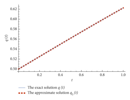
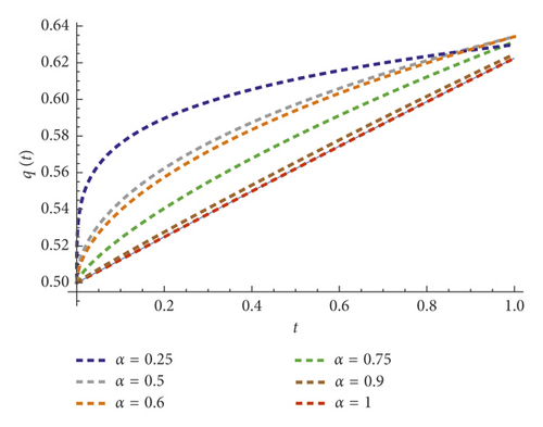
The numerical results of the 5^th FRP solution are given in Table 1 with α = 1 in the interval (0, 1) with step size h = 0.1. Figure 1 shows a comparison between the behavior of the exact solution and the approximate solution at α = 1, while in Table 2, numerical comparison is given between the proposed method and the optimal homotopy asymptotic method (OHAM) [15] at α = 1. In Figure 2, the behavior of the 5^th FPRS approximation is presented with different values of α, where α ∈ {1.0, 0.9, 0.75, 0.5, 0.25} and with step size of 0.2, whereas in Table 3, we review the numerical comparison between the FRPS solutions and the OHAM [15] when α = 1 with step size of 0.3. Anyhow, Table 4 shows the representation of the 6^th approximate solution with different values of α such that α ∈ {1.0, 0.75, 0.5, 0.25}. From these results, it can be observed that the behavior of the approximate solutions for different values of α is in good agreement with each other that depends on the fractional order α.

Table 1. Numerical results of 5^th FRPS at α = 1 for Example 1.

t	Exact solution	Approximations	Absolute error	Relative error
0.1	0.5124973965	0.5124973965	0	0
0.2	0.5249791875	0.5249791875	0	0
0.3	0.5374298453	0.5374298457	3.59375 × 10⁻¹⁰	6.68692 × 10⁻¹⁰
0.4	0.5498339973	0.5498340000	2.68752 × 10⁻⁹	4.88787 × 10⁻⁹
0.5	0.5621765009	0.5621765137	1.27861 × 10⁻⁸	2.27438 × 10⁻⁸
0.6	0.5744425168	0.5744425625	4.56883 × 10⁻⁸	7.95351 × 10⁻⁸
0.7	0.5866175789	0.5866177129	1.33973 × 10⁻⁷	2.28382 × 10⁻⁷
0.8	0.5986876601	0.5986880000	3.39887 × 10⁻⁷	5.67721 × 10⁻⁷
0.9	0.6106392339	0.6106400059	7.71910 × 10⁻⁷	1.26410 × 10⁻⁶

Details are in the caption following the image — **Figure 1**
Open in figure viewer PowerPoint

The behavior of FRPS solution at α = 1 for Example 1.

Table 2. Comparison between the FRPS solutions and the OHAM [15] at α = 1 for Example 1.

t	Exact	Approximations		Absolute error
t	Exact	FRPSM	OHAM	FRPSM	OHAM
0.0	0.5	0.5	0.5	0.00	0.00
0.3	0.5374298453	0.5374298457	0.5374288935	3.59375 × 10⁻¹⁰	9.52 × 10⁻⁷
0.6	0.5744425168	0.5744425625	0.5744461429	4.56883 × 10⁻⁸	3.63 × 10⁻⁶
0.9	0.6106392339	0.6106400059	0.6106416979	7.71910 × 10⁻⁷	2.46 × 10⁻⁶

Table 3. The 5^th FRPS solution of Example 1 for several values t and α.

t	α = 1	α = 0.9	α = 0.75	α = 0.5
0.0	0.5	0.5	0.5	0.5
0.2	0.5249791875	0.5304889353505724	0.5405474790276749	0.5624203934410724
0.4	0.5498340000	0.5566921519428415	0.5678024178207643	0.5873774649503688
0.6	0.5744425625	0.5812250955770806	0.5912278649203895	0.6059542706735661
0.8	0.5986880000	0.6266870034872078	0.6122323913149167	0.6211659591174139
1.0	0.6224609375	0.6266870034872078	0.6314223950369852	0.6341997586473209

Table 4. Representation of approximate solutions for different values of α.

α_i	FPS approximate solution q₆(t)
1/4
1/2
3/4
1	q₆(t) = (1/2) + (1/8)t + (1/384)t³ + (1/15360)t⁵

Example 2. Consider the fractional logistic differential equation

()

with the initial condition

()

The exact solution of IVP (49) and (50) at α = 1 is given by

()

According to the FRPS algorithm, the FPS solution of (49) has the form

()

Now, the residual error of equation (49) can be defined by

()

and the j-th residual function

()

In view of the FRPS algorithm, few terms a_n, n = 1,2,3,4, of equation (52) are given by

()

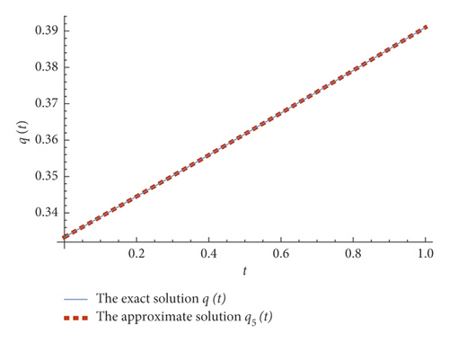
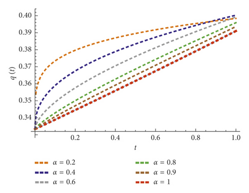
In Table 5, the numerical error of the 5^th FRPS solution is presented for α = 1 on [0,1] with step size of 0.1. In Table 6, the numerical results of the 5^th FRPS solution are given for different values of α on [0,1] with step size of 0.2. The exact and approximate solutions for α = 1, t ∈ [0,1] and n = 5 are shown in Figure 3, while the behaviors of FRPS solutions are plotted for different values of α in Figure 4. From these results, it can be observed that the behavior of the approximate solutions for different values of α is in good agreement with each other that depends on the fractional order α.

Table 5. Numerical results of 5^th FRPS at α = 1 for Example 2.

t	Exact solution	Approximations	Absolute error	Relative error
0.1	0.3389118421	0.3389118421	0	0
0.2	0.3445354618	0.3445354618	1.00 × 10⁻¹¹	3.00 × 10⁻¹¹
0.3	0.3502029635	0.3502029634	1.00 × 10⁻¹⁰	2.00 × 10⁻¹⁰
0.4	0.3559130712	0.3559130706	5.60 × 10⁻⁹	1.50 × 10⁻⁹
0.5	0.3616644631	0.3616644609	2.15 × 10⁻⁸	5.90 × 10⁻⁹
0.6	0.3674557720	0.3674557656	6.40 × 10⁻⁸	1.74 × 10⁻⁸
0.7	0.3732855868	0.3732855706	1.61 × 10⁻⁷	4.33 × 10⁻⁸
0.8	0.3791524531	0.3791524170	3.60 × 10⁻⁷	9.51 × 10⁻⁸
0.9	0.3850548747	0.3850548016	7.31 × 10⁻⁷	1.90 × 10⁻⁷

Table 6. The 5^th FRPS solution of Example 2 for different values of t and α.

t	α = 1	α = 0.9	α = 0.75	α = 0.5
0.0	0.3333333333	0.33333333333	0.33333333333	0.33333333333
0.2	0.3445354618	0.34705266128	0.35171387863	0.36224905383
0.4	0.3559130706	0.35916526544	0.36457322181	0.37469934920
0.6	0.3674557656	0.37084329986	0.37604627351	0.38441631947
0.8	0.3791524170	0.38228876744	0.38673297588	0.39270737781
1.0	0.3909911774	0.39358561694	0.39688357406	0.40007972096

5. Conclusions

This study targets to implement the FRPS method for investigating the approximate solution of fractional logistic system subject to fit initial condition. The target has been accomplished successfully through extending the FRPS algorithm to handle such type of FDEs. The present method provides a solution in rapidly convergent FPS without linearization, or any limitations. Some numerical applications are performed to show the efficiency and reliability of the presented algorithm using Mathematica software package. The obtained results showed that the FRPSM is an easy, efficient, and systematic algorithm to provide analytic series solutions to various emerging systems of science.

Conflicts of Interest

The authors declare that they have no conflicts of interest.

Open Research

Data Availability

The data used to support the findings of this study are available from the corresponding author upon request.

References

1 Oldham K. B. and Spanier J., The Fractional Calculus, 1974, Academic Press, New York, NY, USA.
Google Scholar
2 Podlubny I., Fractional Differential Equations, 1999, Academic Press, New York, NY, USA.
Web of Science® Google Scholar
3 Al-Smadi M. and Arqub O. A., Computational algorithm for solving fredholm time-fractional partial integrodifferential equations of dirichlet functions type with error estimates, Applied Mathematics and Computation. (2019) 342, 280–294, https://doi.org/10.1016/j.amc.2018.09.020, 2-s2.0-85055289577.
10.1016/j.amc.2018.09.020
Web of Science® Google Scholar
4 Abu Arqub O. and Al-Smadi M., Atangana-Baleanu fractional approach to the solutions of Bagley-Torvik and Painlevé equations in Hilbert space, Chaos, Solitons and Fractals. (2018) 117, 161–167, https://doi.org/10.1016/j.chaos.2018.10.013, 2-s2.0-85055338525.
10.1016/j.chaos.2018.10.013
Web of Science® Google Scholar
5 Al-Smadi M., Freihat A., Khalil H., Momani S., and Khan R. A., Numerical multistep approach for solving fractional partial differential equations, International Journal of Computational Methods. (2017) 14, 1–15, 1750029, https://doi.org/10.1142/s0219876217500293, 2-s2.0-84988353691.
10.1142/S0219876217500293
Web of Science® Google Scholar
6 Moaddy K., Freihat A., Al-Smadi M., Abuteen E., and Hashim I., Numerical investigation for handling fractional-order Rabinovich-Fabrikant model using the multistep approach, Soft Computing. (2018) 22, no. 3, 773–782, https://doi.org/10.1007/s00500-016-2378-5, 2-s2.0-84990938451.
10.1007/s00500-016-2378-5
Web of Science® Google Scholar
7 Momani S., Abu Arqub O., Freihat A., and Al-Smadi M., Analytical approximations for Fokker-Planck equations of fractional order in multistep schemes, Applied and Computational Mathematics. (2016) 15, no. 3, 319–330.
Web of Science® Google Scholar
8 Al-Smadi M., Simplified iterative reproducing kernel method for handling time-fractional BVPs with error estimation, Ain Shams Engineering Journal. (2018) 9, no. 4, 2517–2525, https://doi.org/10.1016/j.asej.2017.04.006, 2-s2.0-85026818177.
10.1016/j.asej.2017.04.006
Web of Science® Google Scholar
9 Altawallbeh Z., Al-Smadi M., Komashynska I., and Ateiwi A., Numerical solutions of fractional systems of two-point BVPs by using the iterative reproducing Kernel algorithm, Ukrainian Mathematical Journal. (2018) 70, no. 5, 687–701, https://doi.org/10.1007/s11253-018-1526-8, 2-s2.0-85056814145.
10.1007/s11253-018-1526-8
Web of Science® Google Scholar
10 Al-Smadi M., Freihat A., Hammad M. m. A., Momani S., and Arqub O. A., Analytical approximations of partial differential equations of fractional order with multistep approach, Journal of Computational and Theoretical Nanoscience. (2016) 13, no. 11, 7793–7801, https://doi.org/10.1166/jctn.2016.5780, 2-s2.0-84977651873.
10.1166/jctn.2016.5780
CAS Google Scholar
11 Golmankhaneh A. K. and Cattani C., Fractal logistic equation, Fractal and Fractional. (2019) 3, no. 3, https://doi.org/10.3390/fractalfract3030041.
10.3390/fractalfract3030041
Web of Science® Google Scholar
12 Bhalekar S. and Daftardar-Gejji V., Solving fractional-order logistic equation using a new iterative method, International Journal of Differential Equations. (2012) 2012, 1–12, 975829, https://doi.org/10.1155/2012/975829, 2-s2.0-84881560484.
10.1155/2012/975829
Google Scholar
13 Khader M. M. and Babatin M. M., On approximate solutions for fractional logistic differential equation, Mathematical Problems in Engineering. (2013) 2013, 1–7, 391901, https://doi.org/10.1155/2013/391901, 2-s2.0-84878666959.
10.1155/2013/391901
Web of Science® Google Scholar
14 Sweilam N. H., Khader M. M., and Mahdy A. M. S., Numerical studies for fractional-order Logistic differential equation with two different delays, Journal of Applied Mathematics. (2012) 2012, 1–14, 764894, https://doi.org/10.1155/2012/764894, 2-s2.0-84867762995.
10.1155/2012/764894
Google Scholar
15 Hamarsheh M. and Ismail A. I., Analytical approximation for fractional order logistic equation, International Journal of Pure and Applied Mathematics. (2017) 115, no. 2, 225–245, https://doi.org/10.12732/ijpam.v115i2.3.
10.12732/ijpam.v115i2.3
Google Scholar
16 Al Shammari M., Al-Smadi M., Abu Arqub O., Hashim I., and Alias M. A., Adaptation of residual power series method to solve Fredholm fuzzy integro-differential equations, AIP Conference Proceedings. (2019) 2111, 020002, https://doi.org/10.1063/1.5111209.
10.1063/1.5111209
Google Scholar
17 Moaddy K., Al-Smadi M., and Hashim I., A novel representation of the exact solution for differential algebraic equations system using residual power-series method, Discrete Dynamics in Nature and Society. (2015) 2015, 1–12, 205207, https://doi.org/10.1155/2015/205207, 2-s2.0-84924598922.
10.1155/2015/205207
Web of Science® Google Scholar
18 Alaroud M., Al-Smadi M., Ahmad R. R., and Salma Din U. K., Computational optimization of residual power series algorithm for certain classes of fuzzy fractional differential equations, International Journal of Differential Equations. (2018) 2018, 1–11, 8686502, https://doi.org/10.1155/2018/8686502, 2-s2.0-85050306139.
10.1155/2018/8686502
Google Scholar
19 El-Ajou A., Abu Arqub O., and Al-Smadi M., A general form of the generalized Taylor’s formula with some applications, Applied Mathematics and Computation. (2015) 256, 851–859, https://doi.org/10.1016/j.amc.2015.01.034, 2-s2.0-84923206496.
10.1016/j.amc.2015.01.034
Web of Science® Google Scholar
20 Hasan S., Al-Smadi M., Freihet A., and Momani S., Two computational approaches for solving a fractional obstacle system in Hilbert space, Advances in Difference Equations. (2019) 2019, no. 55, https://doi.org/10.1186/s13662-019-1996-5, 2-s2.0-85061231834.
10.1186/s13662-019-1996-5
PubMed Google Scholar
21 Freihet A., Hasan S., Al-Smadi M., Gaith M., and Momani S., Construction of fractional power series solutions to fractional stiff system using residual functions algorithm, Advances in Difference Equations. (2019) 2019, https://doi.org/10.1186/s13662-019-2042-3, 2-s2.0-85062637227.
10.1186/s13662-019-2042-3
PubMed Google Scholar
22 Alaroud M., Al-Smadi M., Ahmad R. R., and Salma Din U. K., An analytical numerical method for solving fuzzy fractional Volterra integro-differential equations, Symmetry. (2019) 11, no. 2, https://doi.org/10.3390/sym11020205, 2-s2.0-85061845106.
10.3390/sym11020205
Web of Science® Google Scholar
23 Alshammari S., Al-Smadi M., Hashim I., and Alias M. A., Applications of fractional power series approach in solving fractional Volterra integro-differential equations, AIP Conference Proceedings. (2019) 2111, 020003, https://doi.org/10.1063/1.5111210.
10.1063/1.5111210
Google Scholar
24 Baleanu D., Golmankhaneh A. K., and Golmankhaneh A. K., Solving of the fractional non-linear and linear Schrodinger equations by homotopy perturbation method, Romanian Journal of Physics. (2009) 54, 823–832.
CAS Web of Science® Google Scholar
25 Al-Smadi M., Abu Arqub O., and Momani S., A computational method for two-point boundary value problems of fourth-order mixed integrodifferential equations, Mathematical Problems in Engineering. (2013) 2013, 1–10, 832074, https://doi.org/10.1155/2013/832074, 2-s2.0-84877937374.
10.1155/2013/832074
Web of Science® Google Scholar
26 Akgül A., Khan Y., Akgül E. K., Baleanu D., and Al Qurashi M. M., Solutions of nonlinear systems by reproducing kernel method, The Journal of Nonlinear Sciences and Applications. (2017) 10, no. 8, 4408–4417, https://doi.org/10.22436/jnsa.010.08.33.
10.22436/jnsa.010.08.33
Google Scholar
27 Al-Smadi M., Arqub O. A., Shawagfeh N., and Momani S., Numerical investigations for systems of second-order periodic boundary value problems using reproducing kernel method, Applied Mathematics and Computation. (2016) 291, 137–148, https://doi.org/10.1016/j.amc.2016.06.002, 2-s2.0-84978240441.
10.1016/j.amc.2016.06.002
Web of Science® Google Scholar
28 Al-Smadi M., Reliable numerical algorithm for handling fuzzy integral equations of second kind in Hilbert spaces, Filomat. (2019) 33, no. 2, 583–597.
10.2298/FIL1902583A
Web of Science® Google Scholar
29 Al-Smadi M., Abu Arqub O., and El-Ajou A., A numerical iterative method for solving systems of first-order periodic boundary value problems, Journal of Applied Mathematics. (2014) 2014, 1–10, 135465.
10.1155/2014/135465
Google Scholar
30 Akgül A., Inc M., Karatas E., and Baleanu D., Numerical solutions of fractional differential equations of Lane-Emden type by an accurate technique, Advances in Difference Equations. (2015) 2015, https://doi.org/10.1186/s13662-015-0558-8, 2-s2.0-84937912448.
10.1186/s13662-015-0558-8
PubMed Google Scholar
31 Komashynska I. and Al-Smadi M., Iterative reproducing kernel method for solving second-order integrodifferential equations of Fredholm type, Journal of Applied Mathematics. (2014) 2014, 1–11, 459509, https://doi.org/10.1155/2014/459509, 2-s2.0-84901045026.
10.1155/2014/459509
Google Scholar
32 Akgül A., Inc M., and Baleanu D., On solutions of variable-order fractional differential equations, An International Journal of Optimization and Control: Theories and Applications (IJOCTA). (2017) 7, no. 1, 112–116, https://doi.org/10.11121/ijocta.01.2017.00368.
10.11121/ijocta.01.2017.00368
Google Scholar
33 Yang X. J., Generalized local fractional taylor’s formula with local fractional derivative, Journal of Expert Systems. (2012) 1, 26–30.
Google Scholar
34 Golmankhaneh A. K. and Baleanu D., Non-local integrals and derivatives on fractal sets with applications, Open Physics. (2016) 14, no. 1, 542–548, https://doi.org/10.1515/phys-2016-0062, 2-s2.0-85014583679.
10.1515/phys-2016-0062
Web of Science® Google Scholar

Citing Literature

All articles

Advanced Analytical Treatment of Fractional Logistic Equations Based on Residual Error Functions

Abstract

1. Introduction

2. Primary Mathematical Concepts

3. The FRPS Approach

4. Illustrative Examples

5. Conclusions

Conflicts of Interest

Open Research

Data Availability

References

Citing Literature

Figures

References

Information

About Wiley Online Library

Help & Support

Opportunities

Connect with Wiley

Advanced Analytical Treatment of Fractional Logistic Equations Based on Residual Error Functions

Abstract

1. Introduction

2. Primary Mathematical Concepts

3. The FRPS Approach

4. Illustrative Examples

5. Conclusions

Conflicts of Interest

Open Research

Data Availability

References

Citing Literature

Figures

References

Related

Information