Volume 2019, Issue 1 3236093

Research Article

Open Access

Stochastic Analysis of Nonlinear Vehicle-Track Coupled Dynamic System and Its Application in Vehicle Operation Safety Evaluation

Fu-Shan Liu

orcid.org/0000-0001-8058-6694

School of Civil Engineering, Railway Campus, Central South University, 22 Shao-Shan-Nan Road, Changsha, Hunan 410075, China csu.edu.cn

Search for more papers by this author

Zhi-Ping Zeng,

Corresponding Author

Zhi-Ping Zeng

[email protected]

orcid.org/0000-0003-4224-5754

School of Civil Engineering, Railway Campus, Central South University, 22 Shao-Shan-Nan Road, Changsha, Hunan 410075, China csu.edu.cn

Key Laboratory of Engineering Structure of Heavy Haul Railway, Ministry of Education, Central South University, Changsha, Hunan 410075, China csu.edu.cn

Search for more papers by this author

Wei-Dong Wang,

Wei-Dong Wang

School of Civil Engineering, Railway Campus, Central South University, 22 Shao-Shan-Nan Road, Changsha, Hunan 410075, China csu.edu.cn

Key Laboratory of Engineering Structure of Heavy Haul Railway, Ministry of Education, Central South University, Changsha, Hunan 410075, China csu.edu.cn

Search for more papers by this author

Abdulmumin Ahmed Shuaibu,

Abdulmumin Ahmed Shuaibu

School of Civil Engineering, Railway Campus, Central South University, 22 Shao-Shan-Nan Road, Changsha, Hunan 410075, China csu.edu.cn

Engineer, Civil Engineering Department, Ahmadu Bello University, Zaria, Nigeria abu.edu.ng

Search for more papers by this author

Fu-Shan Liu,

Fu-Shan Liu

orcid.org/0000-0001-8058-6694

School of Civil Engineering, Railway Campus, Central South University, 22 Shao-Shan-Nan Road, Changsha, Hunan 410075, China csu.edu.cn

Search for more papers by this author

Zhi-Ping Zeng,

Corresponding Author

Zhi-Ping Zeng

[email protected]

orcid.org/0000-0003-4224-5754

School of Civil Engineering, Railway Campus, Central South University, 22 Shao-Shan-Nan Road, Changsha, Hunan 410075, China csu.edu.cn

Key Laboratory of Engineering Structure of Heavy Haul Railway, Ministry of Education, Central South University, Changsha, Hunan 410075, China csu.edu.cn

Search for more papers by this author

Wei-Dong Wang,

Wei-Dong Wang

School of Civil Engineering, Railway Campus, Central South University, 22 Shao-Shan-Nan Road, Changsha, Hunan 410075, China csu.edu.cn

Key Laboratory of Engineering Structure of Heavy Haul Railway, Ministry of Education, Central South University, Changsha, Hunan 410075, China csu.edu.cn

Search for more papers by this author

Abdulmumin Ahmed Shuaibu,

Abdulmumin Ahmed Shuaibu

School of Civil Engineering, Railway Campus, Central South University, 22 Shao-Shan-Nan Road, Changsha, Hunan 410075, China csu.edu.cn

Engineer, Civil Engineering Department, Ahmadu Bello University, Zaria, Nigeria abu.edu.ng

Search for more papers by this author

First published: 2019

https://doi.org/10.1155/2019/3236093

Citations: 2

Academic Editor: Giuseppe Ruta

Share a link

Email
Wechat
Bluesky

Abstract

This paper presents a vehicle operation safety evaluation model; to this end, a nonlinear vehicle-track coupled dynamic system stochastic analysis model under random irregularity excitations based on probability density evolution method was developed. The nonlinear coupled vehicle-track dynamic system is used to accurately describe the wheel-rail contact state. The stochastic function-spectral representation is used to simulate the random track irregularity in the time domain for the first time; consequently, the frequency components in the irregularity are preserved and random variables are reduced. In the process of evaluating the safety of train operation, the probability evolution, reliability of evaluation indices for different limit values, and evaluation indices for different probability limits are calculated for more accurate evaluation. The dynamic model and safety evaluation method was verified using the Zhai-model and Monte Carlo method. The results show that, when the probability guarantee is increased, the running safety index of the vehicle increases more rapidly with running speed and the left/right wheel-rail derailment coefficient increases rapidly at running speeds above 400 km/h. The computational model provides a novel direction for vehicle operation safety evaluation.

1. Introduction

Vehicle-track coupled dynamic system is a nonlinear and stochastic system in nature as random track irregularity is one of its main random excitations. Meanwhile, the vehicle operation safety under random excitations is also the main transportation engineering concerns. In the past few decades, the popularization of high-speed railway and the continuous demand for high operating speed have brought many engineering challenges. In many countries, evaluation standards for train operation safety have been emplaced. Due to the complexity involved in the safety assessment of train operation, the problems generally need to be addressed through simulation methods. Several different train-track coupled dynamics models or train-bridge coupled dynamics models have been established to analyze the dynamic response of the system. Wu et al. [1] developed a vehicle-rail-bridge interaction model for analyzing the 3D dynamic interaction between the moving trains and railway bridge; in this established model, the wheelset has 3 degrees of freedom, the vertical, lateral, and rolling, and no jumps occur between the wheelsets and rails. After that, Chen and Zhai [2] established two dynamic models, train running on the bridge with ballasted track and the ballastless slab track. In these two models, the jump between the wheelset and the rail can be simulated. In reference [3], Zhai further extended these models to three-dimensional space, and at the same time, a three-dimensional space wheel-rail contact relationship has also been developed. Lou and Zeng [4] have derived the equations of motion in matrix form for the railway freight vehicle-bridge interaction system based on energy approach; this modeling method also has been widely used. Dinh et al. [5] have developed a formulation of three-dimensional dynamic interactions between a bridge and a high-speed train using wheel-rail interfaces; in this model, contact loss is allowed, and the contact is nonlinearly. Other than these, many scholars, such as Zhang et al. [6] and Yang and Yau [7], also have established their own vehicle-track or vehicle-track-bridge coupling dynamics models. The development of vehicle-track coupled dynamics modeling facilitates the evaluation of vehicle operational safety through numerical simulation. However, as the main excitation source in the train operation, the track random irregularity cannot be measured and predicted before the completion of the line construction, it also changes with time and environment. Therefore, it is necessary to consider the train safety operation from a stochastic point of view. Many scholars have tried to use random vibration analysis method to study the dynamic response of vehicle-track coupled dynamic system and have obtained many meaningful research results.

Due to the complexity of vehicle-track coupled dynamic system, Monte Carlo method (MCM) is a common analytical method in random analysis. Chen et al. [8] and Xia et al. [9] studied the random vibrations in a nonlinear vehicle-track coupling dynamic system by the MCM and established an early nonlinear analysis model of the system from a stochastic perspective. Subsequently, many efficient random vibration methods were applied to vehicle-track-coupled power systems. Lu et al. [11], Zhang et al. [12], and Zeng et al. [13] established random vibration analysis model for linear vehicle-track-bridge coupling system by pseudoexcitation method (PEM). This method analyzes the random vibrations in linear systems efficiently, especially the power characteristics in the frequency domain. Zhang et al. also have used the PEM and the precise integration method (PIM) to compute the nonstationary random responses of three-dimensional train-bridge systems subjected to lateral horizontal earthquakes [14]. Yu et al. [15] studied the random vibrations of a linearized vehicle-rail-bridge coupling system by generalized probability density evolution theory (originally formulated by Li and Chen [16]), which is more efficient than the MCM. Xu et al. [17, 18] proposed a stochastic space-time analysis method for vehicle-track-coupled power systems. Their method also applies generalized probability density evolution theory and is based on the measured track irregularity data. Their probabilistic model efficiently and accurately analyzes the vehicle-track-coupled power system under random track irregularities.

The introduction of stochastic vibration analysis method makes it possible to use the probability theory to evaluate the safety of vehicle-track coupled power system or vehicle-bridge coupled dynamic system. Rocha et al. presented a probabilistic methodology for the safety assessment of short-span railway bridges for high-speed traffic [19] and analysed the sensitivity of the dynamic response due to the variability of the main structural parameters [20], and the efficiency of different probabilistic methodologies for safety assessment of short-span railway bridges is compared [21]. Using the principle of virtual work, utilizing a linearized wheel-rail contact equation to avoid iterative solution at each time step of the integration, and applying rail irregularity as random excitations to the system, the probabilistic evaluation approach for nonlinear vehicle-bridge dynamic performances has been analysed by Jin et al. [22]. By developing an improved response surface method for nonlinear limit states, Cho et al. [23] evaluated the reliability of vehicle and high-speed railway bridge system.

In the existing random vibration analysis of vehicle-track coupled dynamics, due to the limitation of stochastic analysis methods or in order to improve the computational efficiency, linear or linearized models are often used. For the linearization of a model, the wheel-rail relationship is often reduced to a linear model. The wheel-rail relationship not only reflects the force state between wheel and rail, but also the excitation of track irregularity also needs to be input into the system through wheel-rail relationship; this makes the wheel-rail relationship one of the core issues in the modeling. The linearized model will not be able to accurately simulate the change of the size, direction, and action point of the wheel-rail force, and it will also lead to a difference of the input track irregularity excitation input. Other than this, models with nonlinear wheel-rail contact relationship allow for the evaluation of vehicle safety in a more realistic way than linear methods [24]. Numerous studies on vehicle-bridge dynamics have indicated that nonlinear interaction has profound effects on the system responses [25]. Therefore, the nonlinear vehicle-track coupled dynamics model is more helpful for vehicle-safety evaluation, and the calculation results are more accurate.

In this paper, a stochastic analysis model of nonlinear vehicle-track coupled dynamic system under random irregularity excitations was established based on probability density evolution method. The nonlinear wheel-rail relationship has been considered to facilitate more convenient and accurate evaluation of vehicle operational safety. Generalized probability density evolution theory has been used, which has been widely applied to linear and nonlinear stochastic systems and have proven to obviously improve the efficiency the analysis [15, 16, 26]. In addition, function-spectral representation method has been used to accurately simulate the random track irregularities in the time domain, which retains a large number of frequency components in the samples while reducing the required number of random variables. It also avoids the clustering phenomenon in the point selection of high-dimensional random variables. The probability density evolution of the left/right wheel-rail load reduction, the left/right wheel-rail derailment coefficient, and the vertical/transverse acceleration of the car body were calculated by the generalized probability density evolution theory. Based on the results, a safety evaluation model of train operation is presented and validated by comparison with previous study. The developed computational model provides a new research direction for train safety evaluation.

2. Stochastic Analysis Model of Nonlinear Vehicle-Track Coupled Dynamic System

Figure 1 shows the calculation flow of the nonlinear vehicle-track coupled dynamic system stochastic analysis model, which is based on generalized probability density evolution theory. The main steps are the establishment of the nonlinear system, the numerical simulation of N_pt random track irregularities time-domain samples, the dynamic response calculation of the coupled vehicle-track system under random excitations, calculation of the probability density evolution of the safety evaluation index, and the train safety evaluation.

Details are in the caption following the image — **Figure 1**
Open in figure viewer PowerPoint

Flow chart of the method for evaluating train operation safety.

2.1. Stochastic Analysis Method Based on Generalized Probability Density Evolution Theory

2.1.1. Generalized Probability Density Evolution Theory

Under random irregular excitations, the nonlinear vehicle-track coupled dynamic system is expressed as

\begin{matrix} [M] \ddot{ξ} (t) + [C] \dot{ξ} (t) + [K] ξ (t) = F (Θ, t), \end{matrix}

(1)

where t denotes time, and ξ(t),

\dot{ξ} (t)

\ddot{ξ} (t)

are the displacement, velocity, and acceleration vectors of the coupled system, respectively. The matrices [M], [C], and [K] are the mass, damping, and stiffness matrices, respectively, reflecting the mechanical and geometric nonlinearity in the wheel-rail relationship. F(Θ, t) is the input excitation vector of track random irregularities, and Θ is the set of sampled random variables.

Most of the randomness in a vehicle-track coupled dynamic system derives from the random track irregularities. A nonlinear vehicle-track dynamic system ξ (t) is a probabilistic conservative stochastic system that excludes other random sources. According to the probabilistic conservation principle of stochastic systems, probabilistic conservation-augmented systems are constructed as [ξ (t), Θ] with

\begin{matrix} P \{(ξ (t), Θ) \in (Ω_{t} \times Ω_{θ})\} = P \{(ξ (t_{0}), Θ) \in (Ω_{t_{0}} \times Ω_{θ})\}, \end{matrix}

(2)

where P{·} denotes the probability of random events. Ω_t and

Ω_{t_{0}}

are the time distribution regions of the system state at times t and t₀, respectively, and Ω_θ is the space distribution region of the system state of sample θ. The above expression is equivalent to

\begin{matrix} \frac{d}{d t} P \{(ξ (t), Θ) \in (Ω_{t} \times Ω_{θ})\} = 0. \end{matrix}

(3)

Expressing the joint probability density function (ξ(t), Θ) as p_ξθ(ξ, θ, t), the above expression becomes

\begin{matrix} \frac{D}{D_{t}} \int_{Ω_{t} \times Ω_{θ}} p_{ξ_{Θ}} (ξ, θ, t) d ξ d θ = 0, \end{matrix}

(4)

where D/D_t is the derivative of matter [16].

The generalized probability density evolves by the following equation [16]:

\begin{matrix} \frac{\partial p_{ξ_{Θ}} (ξ, θ, t)}{\partial t} + \dot{ξ} (θ, t) \frac{\partial p_{ξ_{Θ}} (ξ, θ, t)}{\partial ξ} = 0. \end{matrix}

(5)

In this formula, $\dot{ξ} (θ, t)$ is the free velocity of ξ (t) under the random sample {Θ = θ}. Its initial probability is ${P_{ξ_{Θ}} (ξ, θ, t)|}_{t = 0} = δ (ξ - ξ_{0}) P_{Θ} (θ)$ .

Solving the above evolution equation of generalized probability density under the initial conditions, we obtain the joint probability density function of sample θ, p_ξΘ(ξ, θ, t). Furthermore, the probability density function of P_ξΘ is obtained by integrating θ:

\begin{matrix} P_{ξ Θ} (ξ, t) = \int_{Ω_{Θ}} p_{ξ Θ} (ξ, θ, t) d θ . \end{matrix}

(6)

For the probabilistic conservative vehicle-track coupled dynamic system under the random track irregularity excitation, the system dynamic response ξ satisfies the generalized probability density evolution equation shown in equation (5). Simultaneously, the generalized probability density evolution equation decouples the probability space from the physical space. As shown in Figure 1, first solve the vehicle-track coupled dynamic system equation (1) to obtain $\dot{ξ} (θ, t)$ under each random sample θ, and then solve the generalized probability density evolution equation for each random sample θ. When all random samples have been calculated, by solving equation (6), the probability density evolution process of the dynamic response can be obtained. Finally, a stochastic analysis of the nonlinear vehicle-track coupled dynamic system is realized.

2.1.2. Selection of Random Variable Samples and the Probability Assignment

In generalized probability density evolution theory, selecting the random variable samples is directly related to the computational efficiency of the random analysis. In this paper, the random variables are described by a low-deviation sequence selected by number theory, which reduces the required number of random samples and accelerates the convergence of the calculation. However, as the low-deviation sequence is uniformly distributed, it cannot be selected from a high-dimensional space without forming void and cluster structures. Therefore, the uniformity will degrade and the calculation results will contain large errors.

Random irregularity is the superposition of irregular waves of different wavelengths, different phases, and different amplitudes. To accurately simulate the random track irregularities, more random frequencies and phase components (i.e., more selections) are needed. To avoid clustering in the random sample selection, the random track irregularities were simulated in the time domain by a stochastic function-spectral representation method, which requires just eight random variables. The generation method and validation of the sampling will be discussed in Section 2.4. The random variables were sampled as Sobol sequences.

The random samples in the probabilistic space Ω_Θ must then be divided. Probabilistic spaces are commonly divided into representative Voronoi regions with representative volumes V (θ_k) satisfying

\begin{matrix} ⋃_{k}^{N_{p t}} V (θ_{k}) = Ω_{Θ}, \\ V (θ_{i}) \cap V (θ_{j}), i \neq j . \end{matrix}

(7)

The assigned probability P_k of random sample θ_k is given by

\begin{matrix} P_{k} = \int_{V (θ_{k})} p_{Θ} (θ_{k}) d v, \end{matrix}

(8)

where p_Θ(θ_k) is the probability density of random variable Θ in Voronoi region V(θ_k). The joint probability density in the total partitioned space satisfies

\begin{matrix} \sum_{k = 1}^{N_{p t}} P_{k} = \sum_{k = 1}^{N_{p t}} \int_{V (θ_{k})} p_{Θ} (θ_{k}) d v = 1 . \end{matrix}

(9)

This method obtains the initial probability of each random point sample.

2.2. Vehicle-Track Coupled Dynamics Model

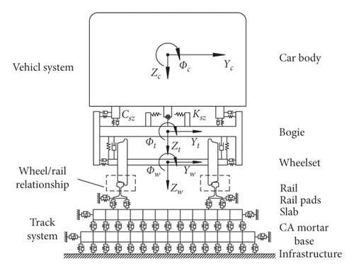
Figure 2 shows the vehicle-track coupling dynamic model. The vehicle is modeled by multirigid body dynamics, and the rail is regarded as a finite-length, elastic-point supported Euler beam. The dynamic vibration equation of the beam is solved by the Ritz method. The wheel-rail relationship is modeled by nonlinear Hertz contact theory and wheel-rail nonlinear creep theory. The fastener is modeled by a linear spring damping element in the transverse and vertical directions. The track structure is modeled by the finite element method; the slab, mortar layer, and base are modeled as plate elements. The foundation support is simplified as a linear spring damping surface element. The wheel-rail relationship connects the vehicle and rail models, whereas the fastener force connects the rail model and the track slab-foundation structure.

2.2.1. Vehicle Dynamics Model

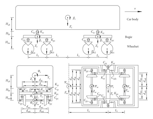
Figure 3 schematizes the vehicle model composed of one car body, two bogies, and four wheelsets. Each part is treated as a rigid body with freedom in the longitudinal, transverse, bounce, roll, and yaw directions (giving 35 degrees of freedom per vehicle).

The antisnake shock absorber significantly affects the driving quality when the train is running at a high speed. Treating the force of the antisnake shock absorber on the vehicle and the antirolling moment of the vehicle’s central suspension as an additional force on the vehicle, the dynamic equation of the vehicle is given by

\begin{matrix} [M_{V}] {\ddot{ξ}}_{V} + [C_{V}] {\dot{ξ}}_{V} + [K_{V}] ξ_{V} + [G_{V}] = [F_{V}], \end{matrix}

(10)

where [M_V], [C_V], [K_V], [G_V], [F_V] are the vehicle mass, damping, stiffness, additional force, and load matrices, respectively.

The freedom matrix of the vehicle is expressed as

\begin{matrix} [ξ_{V}] = {[ξ_{c}, ξ_{b 1}, ξ_{b 2}, ξ_{w 1}, ξ_{w 2}, ξ_{w 3}, ξ_{w 4}]}^{T}, \end{matrix}

(11)

where the subscripts c, b, and w represent the car body, bogie, and wheelset, respectively, and the subscripts i and j represent the ith bogie and the jth wheelset, respectively. The degrees of freedom of each part are expressed as

\begin{matrix} ξ_{c, b i, w j} = [Y_{c, b i, w j}, Z_{c, b i, w j}, ψ_{c, b i, w j}, β_{c, b i, w j}, φ_{c, b i, w j}], \end{matrix}

(12)

where Y, Z, Ψ, φ, and β represent the freedoms in the longitudinal, transverse, bounce, roll, and yaw, respectively.

The vehicle-mass matrix is given by

\begin{matrix} [M_{V}] = [M_{w 1}, M_{w 2}, M_{w 3}, M_{w 4}, M_{t 1}, M_{t 2}, M_{c}], \end{matrix}

(13)

where M_wi,bj,c = diag[m_wi,bj,c, m_wi,bj,c, Ix_wi,bj,c, Iy_wi,bj,c, Iz_wi,bj,c]. Here m denotes the mass, and Ix, Iy, and Iz are the moments of inertia around the X, Y, and Z axes, respectively.

The vehicle-stiffness matrix is given by

\begin{matrix} [K_{V}] = [\begin{matrix} K_{w 1} & 0 & 0 & 0 & K_{w b 1} & 0 & 0 \\ K_{w 2} & 0 & 0 & K_{w b 2} & 0 & 0 \\ K_{w 3} & 0 & 0 & K_{w b 3} & 0 \\ K_{w 4} & 0 & K_{w b 4} & 0 \\ K_{b 1} & 0 & K_{b c 1} \\ K_{b 2} & K_{b c 2} \\ syms & K_{c} \end{matrix}], \end{matrix}

(14)

where

\begin{matrix} K_{w i} = 21,2,3,4 [\begin{matrix} k_{p y} \\ k_{p z} \\ k_{p z} d_{w}^{2} \\ 0 \\ k_{p x} d_{w}^{2} \end{matrix}], i =, \\ K_{b j} = 2 [\begin{matrix} 2 k_{p y} + k_{s y} & 0 & - 2 k_{p y} H_{t w} + k_{s y} H_{b t} & 0 & 0 \\ 2 k_{p z} + k_{s z} & 0 & 0 & 0 \\ 22 k_{p y} H_{t w}^{2} + k_{p z} d_{w k}^{2} + k_{s z} d_{s k}^{2} + k_{s y} H_{b t}^{2} & 0 & 0 \\ 22 k_{p z} l_{t}^{2} + k_{p x} H_{t w}^{2} + k_{s x} H_{b t}^{2} & 0 \\ syms & 22 k_{p y} l_{t}^{2} + k_{p x} d_{w k}^{2} + k_{s x} d_{s k}^{2} \end{matrix}], \\ K_{c} = 4 [\begin{matrix} k_{s y} & 0 & - k_{s y} H_{c b} & 0 & 0 \\ k_{s z} & 0 & 0 & 0 \\ k_{s y} H_{c b}^{2} + k_{s z} d_{s k}^{2} & 0 & 0 \\ k_{s z} l_{c}^{2} + k_{s x} H_{c b}^{2} & 0 \\ syms & k_{s y} l_{c}^{2} + k_{s x} d_{s k}^{2} \end{matrix}], \\ K_{w b i} = 21,2,3,4, [\begin{matrix} - k_{p y} & 0 & k_{p y} H_{t w} & 0 & {(- 1)}^{i} k_{p y} l_{t} \\ - k_{p z} & 0 & {(- 1)}^{i + 1} k_{p z} l_{t} & 0 \\ - k_{p z} d_{w k}^{2} & 0 & 0 \\ 0 & 0 \\ syms & - k_{p x} d_{w k}^{2} \end{matrix}], i = \\ K_{b c j} = 21,2. [\begin{matrix} - k_{s y} & 0 & k_{s y} H_{c b} & 0 & {(- 1)}^{j + 1} k_{s y} l_{c} \\ - k_{s z} & 0 & {(- 1)}^{j + 1} k_{s z} l_{c} & 0 \\ - k_{s z} d_{s k}^{2} + k_{s y} H_{c b} H_{b t} & 0 & {(- 1)}^{j} k_{s y} l_{c} H_{b t} \\ k_{s x} H_{c b} H_{b t} & 0 \\ syms & - k_{s x} d_{s k}^{2} \end{matrix}], j = \end{matrix}

(15)

The vehicle-damping matrix

\begin{matrix} [C_{V}] = [\begin{matrix} C_{w 1} & 0 & 0 & 0 & C_{w b 1} & 0 & 0 \\ C_{w 2} & 0 & 0 & C_{w b 2} & 0 & 0 \\ C_{w 3} & 0 & 0 & C_{w b 3} & 0 \\ C_{w 4} & 0 & C_{w b 4} & 0 \\ C_{b 1} & 0 & C_{b c 1} \\ C_{b 2} & C_{b c 2} \\ syms & C_{c} \end{matrix}], \end{matrix}

(16)

is similar to the vehicle-stiffness matrix. In fact, the vehicle-damping matrix is obtained by replacing the stiffness values in the stiffness matrix with the corresponding damping values.

The additional moment on the vehicle is expressed as the matrix

\begin{matrix} [G] = [G_{w 1}, G_{w 2}, G_{w 3}, G_{w 4}, G_{t 1}, G_{t 2}, G_{c}], \end{matrix}

(17)

with

\begin{matrix} G_{w i} = {[0,00, I y_{w i} ({\dot{β}}_{w i} - Ω) {\dot{φ}}_{w i},, I y_{w i} ({\dot{β}}_{w i} - Ω) {\dot{ψ}}_{w i}]}^{T}, \\ G_{t j} = {[0,0,0, [F_{x s L j} + F_{x s R j}] H_{b t}, [F_{x s L j} - F_{x s R j}] d_{s x}]}^{T}, \\ G_{c} = [0,0, M_{r 1} + M_{r 2}, (F_{x s L 1} + F_{x s R 1} + F_{x s L 2} + F_{x s R 2}) H_{c b}, (F_{x s L 1} + F_{x s L 2} - F_{x s R 1} - F_{x s R 2}) d_{s x}] . \end{matrix}

(18)

In the above expressions, G_wi is the matrix of moments acting on the ith wheelset caused by wheelset rolling rotations, G_tj is the matrix of moments acting on the jth bioge caused by absorber, G_c is the matrix of moments acting on the car body caused by absorber, and F_xsLj and F_xsLj are the additional forces imposed by the snake-shaped shock absorber. They are calculated as follows:

\begin{matrix} F_{x s (L, R) j} = \{\begin{cases} \frac{F_{\max} v_{x c t (L, R) j}}{v_{0}}, & |v_{x c t (L, R) j}| < v_{0}, \\ F_{\max} sign (v_{x c t (L, R) j}), & |v_{x c t (L, R) j}| \geq v_{0} . \end{cases} \end{matrix}

(19)

M_ri is the antiroll moment, given by

\begin{matrix} M_{r i} = K_{r x} (ψ_{c} - ψ_{t i}), i = 1,2. \end{matrix}

(20)

The vehicle-load matrix is expressed as

\begin{matrix} F = [A_{1} F_{w r 1}, A_{2} F_{w r 2}, A_{3} F_{w r 3}, A_{4} F_{w r 4}, 0_{51 \times}, 0_{51 \times}, 0_{51 \times}], \end{matrix}

(21)

where A_i is the matrix of conversion coefficients between the wheel-rail force and the vehicle freedoms. F_wri is the wheel-rail force array, with

\begin{matrix} A_{w i} = [\begin{matrix} 0 & 1 & 0 & 1 & 0 & 0 & 0 & 0 & 0 & 0 & 0 & 0 \\ 0 & 0 & - 1 & 0 & 0 & - 1 & 0 & 0 & 0 & 0 & 0 & 0 \\ 0 & - r_{L i} & a_{0} & 0 & - r_{L i} & - a_{0} & 0 & 0 & 0 & 0 & 0 & 0 \\ r_{L i} & r_{L i} φ_{w i} & 0 & r_{R i} & r_{R i} φ_{w i} & 0 & 0 & 1 & 0 & 0 & 1 & 0 \\ a_{0} & a_{0} φ_{w i} & 0 & - a_{0} & - a_{0} φ_{w i} & 0 & 0 & 0 & 1 & 0 & 0 & 1 \end{matrix}], \\ F_{w r i} = [F_{L x i}, F_{L y i}, F_{L z i}, F_{R x i}, F_{R y i}, F_{R z i}, M_{c L x i}, M_{c L y i}, M_{c L z i}, M_{c R x i}, M_{c R y i}, M_{c R z i}], \end{matrix}

(22)

where F_L,Rxi = F_nL,Rxi + F_cL,Rxi, F_L,Ryi = F_nL,Ryi + F_cL,Ryi, and F_L,Rzi = F_nL,Rzi + F_cL,Rzi. F_n and F_c are the normal and creep forces, respectively, between the wheel and the rail. The subscripts L and R represent the left and right sides, respectively, and the subscripts x, y, and z denote the upper component in the X-, Y-, and Z-axis directions, respectively.

2.2.2. Dynamic Model of the Track Structure

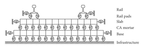
The track structure is divided into two main parts: the rail and the track plate. The rail is treated as an elastic support for an Euler beam, and the track plate and base plate are modeled by a plate element with high rigidity in the transverse direction, lateral displacement using beam element to simulate. Since the numerical integration solution step length is short and requires a lot of numerical calculation work, the method of the literature [3] is used in the modeling of the rail, and the dynamic response of the rail is obtained by solving the rail vibration differential equation, which can greatly reduce the calculation work. At the same time, the track plate is modeled by the finite element method to facilitate the modeling of various ballastless track structures. The track-structure model and rail forces are shown in Figures 4 and 5, respectively.

The following expressions are shown for the right rail (the left rail is treated analogously). The fastener force matrix is expressed as

\begin{matrix} [\begin{matrix} F_{p v i} \\ F_{p h i} \\ M_{p i} \end{matrix}] = [\begin{matrix} 0 & k_{p v} & 0 & 0 & - k_{p v} \\ k_{p h} & 0 & k_{p h} H_{r a} & - k_{p h} & 0 \\ - k_{p h} H_{r a} & 0 & k_{p h} H_{r a}^{2} + k_{p v} L_{r}^{2} & k_{p h} H_{r a} & 0 \end{matrix}] {[Y_{r i}, Z_{r i}, ψ_{r i}, Y_{s i}, Z_{s i}]}^{T} . \end{matrix}

(23)

The torque of the wheel-rail force, which induces rail torsion, is

\begin{matrix} M_{c r} = F_{R y} H_{r b} - F_{R z} L_{c e} . \end{matrix}

(24)

The differential equations of the vertical, transverse, and torsional vibrations of the rail are, respectively given in the following [3].

Vertical:

\begin{matrix} E I_{r z} \frac{\partial^{4} Y_{r} (x, t)}{\partial x^{4}} + m_{r} \frac{\partial^{2} Y_{r} (x, t)}{\partial t^{2}} = - \sum_{i = 1}^{N} F_{p y i} (t) δ (x - x_{i}) + \sum_{j = 1}^{4} F_{R y j} (t) δ (x - x_{w j}) . \end{matrix}

(25)

Transverse:

\begin{matrix} E_{r} I_{r z} \frac{\partial^{4} Z_{r} (x, t)}{\partial x^{4}} + m_{r} \frac{\partial^{2} Z_{r} (x, t)}{\partial t^{2}} = - \sum_{i = 1}^{N} F_{p v i} (t) δ (x - x_{i}) + \sum_{i = 1}^{4} F_{R z j} (t) δ (x - x_{w j}) . \end{matrix}

(26)

Torsional:

\begin{matrix} ρ_{r} I_{r 0} \frac{\partial^{2} ψ_{r} (x, t)}{\partial t^{4}} - G_{r} I_{t} \frac{\partial^{2} ψ_{r} (x, t)}{\partial x^{2}} = - \sum_{i = 1}^{N} M_{p i} (t) δ (x - x_{i}) + \sum_{j = 1}^{4} M_{c r j} (t) δ (x - x_{w j}) . \end{matrix}

(27)

The track and base plates are considered as horizontally rigid bodies and are modeled as four-node bending plate elements. They are connected by a fastener element, which is simulated by a linear spring damping element. Slab-base has been modeled by the principle of total potential energy with stationary value in elastic system dynamics [4], the dynamics of the slab and base plates are governed by

\begin{matrix} [\begin{matrix} M_{s s} \\ M_{b b} \end{matrix}] [\begin{matrix} {\ddot{δ}}_{s} \\ {\ddot{δ}}_{b} \end{matrix}] + [\begin{matrix} C_{s s} & C_{s b} \\ C_{b s} & C_{b b} \end{matrix}] [\begin{matrix} {\dot{δ}}_{s} \\ {\dot{δ}}_{b} \end{matrix}] + [\begin{matrix} K_{s s} & K_{s b} \\ K_{b s} & K_{b b} \end{matrix}] [\begin{matrix} δ_{s} \\ δ_{b} \end{matrix}] = [\begin{matrix} F_{s} \\ F_{b} \end{matrix}], \end{matrix}

(28)

where the subscript s and b denote the track and base plates, respectively. The vibration equation of the track and base plates assumes the principle of invariant potential energy of an elastic system. The foundation structure is modeled by the same method. [F] is the load matrix, and the main load acting on the slab-base is the fastening force. The matrix and modeling process of the track and base plates are detailed elsewhere [13].

2.2.3. Wheel-Rail Contact Relation

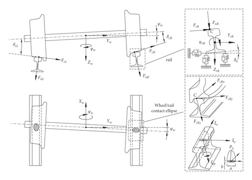
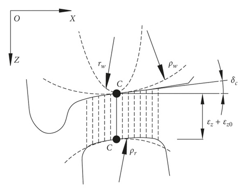
The wheel-rail relationship links the vehicle system to the track system. In the vehicle-track coupled dynamics, the wheel-rail relationship mainly includes the wheel-rail normal-seeking solution, the wheel-rail creep solution, and the wheel-rail contact geometry. The wheel-rail relationship is shown in Figure 6.

(1) The Wheel-Rail Normal Contact Model. The wheel tread and rail profile are complex curves composed of many simple curves with different radii. According to nonlinear Hertz contact theory (Figure 7), the shapes of the wheel and rail tread near the contact point are approximately described as

\begin{matrix} z_{1} = \frac{1}{2 ρ_{w}} x_{1}^{2} + \frac{1}{2 r_{w}} y_{1}^{2}, for the wheel tread, \\ z_{2} = - \frac{1}{2 ρ_{r}} x_{2}^{2}, for the rail tread, \end{matrix}

(29)

where r_p, r_w, and r_r represent the curvature radii of the wheel tread, wheel rolling circle, and rail tread, respectively. Positive and negative curvatures indicate a convex and concave surface, respectively.

The pressure distribution on the contact surface is given by Hertz contact theory.

\begin{matrix} p = P_{n} {[1 - {(\frac{x}{a})}^{2} - {(\frac{y}{b})}^{2}]}^{12 /} . \end{matrix}

(30)

The normal force on the wheel and rail is expressed as

\begin{matrix} F_{n L, R} = \frac{4}{3} E^{*} R_{e}^{12 /} {(\frac{ε_{n L, R}}{F_{2} (e)})}^{32 /} . \end{matrix}

(31)

And the maximum pressure between the wheel and rail is given by

\begin{matrix} P_{n L, R} = {(\frac{6 F_{n L, R} E^{* 2}}{π^{3} R_{e}^{2}})}^{13 /} {[F_{1} (e)]}^{- 2} . \end{matrix}

(32)

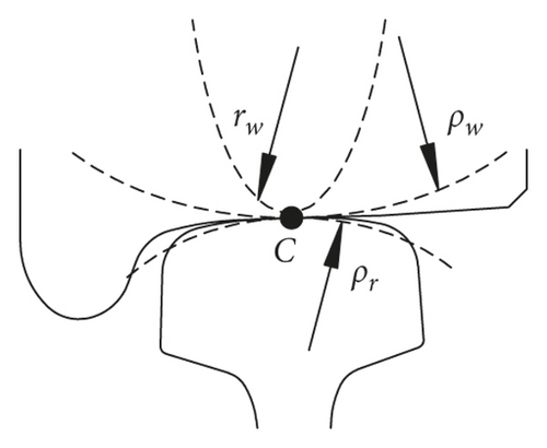
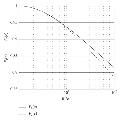
In the above expressions, E^∗ is the equivalent modulus of elasticity, given by $1 / E^{*} = (1 - v_{r}^{2}) / E_{r} + (1 - v_{w}^{2}) / E_{w}$ , and $e = {((1 - b^{2}) / a^{2})}^{12 /}$ , where a and b are the lengths of the long and short axes, respectively, of the contact ellipse (with b < a). F₁(e) and F₂(e) are correction factors that depend only on the ratio of relative curvature radii R^′/R^″. The variations of these factors with increasing R^′/R^″ are plotted in Figure 8.

F ₁(e) and F₂(e) can be directly computed by a formula or directly read from Figure 9. To improve the efficiency of the computation, the curve-fitting parameters obtained from Figure 9 are listed in Table 1, F₁(e) and F₂(e) were then obtained as

\begin{matrix} F_{i} (e) = \frac{q_{1} x^{5} + q_{2} x^{4} + q_{3} x^{3} + q_{4} x^{2} + q_{5} x^{1} + q_{6}}{x^{3} + p_{1} x^{2} + q_{2} x^{1} + q_{3}}, \end{matrix}

(33)

with x = ln(B/A).

Table 1. Fitting parameters of the F₁(e) and F₂(e) curves.

F₁(e)			F₂(e)
Parameters		Error of fitting	Parameters		Error of fitting
q₁	0.001227	SSE: 3.522e-07	q₁	0.002195	SSE: 3.156e-07
q₂	−0.05683	R-square: 1	q₂	−0.07143	R-square: 1
q₃	0.7315	Adjusted R-square: 1	q₃	0.4331	Adjusted R-square: 1
q₄	4.087	RMSE: 5.935e-07	q₄	4.816	RMSE: 5.618e-07
q₅	20.1		q₅	41.2
q₆	36.46		q₆	21.94
p₁	4.599		p₁	5.123
p₂	20.1		p₂	41.2
p₃	36.46		p₃	21.94

When calculating the normal contact force between the wheel and rail, the relative compression between the wheel and a rail with random irregularities is obtained by geometrically solving the wheel-rail contact. The normal force between the wheel and rail is then obtained by solving the wheel-rail normal contact model and determining the direction and magnitude variations in the normal wheel-rail force at different contact points. Converting to the absolute coordinate system, the normal loads on the wheel and rail array are, respectively, expressed as

\begin{matrix} F_{n L i}^{'} = {[F_{n L x i}, F_{n L y i}, F_{n L z i}]}^{T} = F_{n L i} {[\sin (δ_{c L i} + ψ_{w i}) \sin (φ_{w i}), - \sin (δ_{c L i} + ψ_{w i}) \cos (φ_{w i}), \cos (δ_{c L i} + ψ_{w i})]}^{T}, \\ F_{n R i}^{'} = {[F_{n R x i}, F_{n R y i}, F_{n R z i}]}^{T} = F_{n R i} {[- \sin (δ_{c R i} - ψ_{w i}) \sin (φ_{w i}), \sin (δ_{c R i} - ψ_{w i}) \cos (φ_{w i}), \cos (δ_{c R i} - ψ_{w i})]}^{T} . \end{matrix}

(34)

Here, δ_cLi and δ_cRi are the left-sided and right-sided wheel-rail contact angles, respectively, obtained from the wheel-rail contact geometry (details will be given in Section (2)).

(2) Wheel-Rail Tangential Contact Model. The wheel-rail tangential contact was solved by Kalker linear creep theory [27], corrected for nonlinearity. The creep force and creep torque between the wheel and rail after the nonlinear correction are given by

\begin{matrix} \{\begin{cases} F_{x}^{'} = α \cdot F_{x}, \\ F_{y}^{'} = α \cdot F_{y}, \\ M_{z}^{'} = α \cdot M_{z}, \end{cases} \end{matrix}

(35)

where α is the correction coefficient, given as

α = F_{R}^{'} / F_{R}

with

F_{R} = \sqrt{F_{x}^{2} + F_{y}^{2}}

and

\begin{matrix} F_{R}^{'} = \{\begin{cases} μ F_{n L, R} [\frac{F_{R}}{μ F_{n L, R}} - \frac{1}{3} {(\frac{F_{R}}{μ F_{n L, R}})}^{2} + \frac{1}{27} {(\frac{F_{R}}{μ F_{n L, R}})}^{3}], & F_{R} \leq 3 μ F_{n L, R}, \\ μ F_{n L, R}, & F_{R} > 3 μ F_{n L, R}, \end{cases} \end{matrix}

(36)

F_x and F_y denote the creep forces in the X- and Y-axis directions, respectively, and M_z is the rotational creep moment. In linear creep theory, these components are, respectively, expressed as

\begin{matrix} \{\begin{cases} F_{x} = - f_{11} ξ_{x}, \\ F_{y} = - f_{22} ξ_{y} - f_{23} ξ_{s p}, \\ M_{z} = f_{23} ξ_{y} - f_{23} ξ_{s p}, \end{cases} \end{matrix}

(37)

where f₁₁ and f₂₂ are the longitudinal and transverse creep coefficients, respectively, and f₂₃ and f₃₃ are rotational creep coefficients:

\begin{matrix} \{\begin{cases} f_{11} = G_{w r} (a b) C_{11}, \\ f_{22} = G_{w r} (a b) C_{22}, \\ f_{23} = G_{w r} {(a b)}^{32 /} C_{23}, \\ f_{33} = G_{w r} {(a b)}^{2} C_{33} . \end{cases} \end{matrix}

(38)

In the above expressions, G_wr is the composite shear modulus of the wheel and rail materials, and C_ij are the Kalker coefficients [27] (after Kalker, who calculated them). Meymandet al. [28] have fitted the Kalker coefficients under different contact conditions. Here, the C_ijs are expressed as

\begin{matrix} \{\begin{cases} C_{11} = 2.392.3381.0142.7360.07280.0139 + v_{w r} + g + v_{w r}^{2} - v_{w r} g - g^{2}, \\ C_{22} = 2.3530.02121.0741.1630.0319 - v_{w r} + g + v_{w r} g - g^{2}, \\ C_{23} = 0.28660.44671.0490.0380.01770.0050.1479 + v_{w r} + g + v_{w r} g - g^{2} + g^{3} + g^{2} v_{w r}, \\ C_{33} = 0.73751.1770.45061.0760.023 - v_{w r} + (\frac{1}{g}) + v_{w r} (\frac{1}{g}) - {(\frac{1}{g})}^{2}, \end{cases} \end{matrix}

(39)

where g is the ratio of the long- and short-elliptical axes, g = a/b, and v_wr is the equivalent Poisson’s ratio.

The calculated creep force and creep torque between the wheel and rail needs to be converted to the absolute coordinate system. The load array of the wheel-rail creep force is expressed as

\begin{matrix} F_{c w r L i} = {[F_{c L x i}, F_{c L y i}, F_{c L z i}]}^{T} = [C_{w r L i}] \cdot {[F_{x L i}, F_{y L i}, 0]}^{T}, \\ F_{c w r R i} = {[F_{c R x i}, F_{c R y i}, F_{c R z i}]}^{T} = [C_{w r R i}] \cdot {[F_{x R i}, F_{y R i}, 0]}^{T}, \\ M_{c w r L i} = {[M_{c L x i}, M_{c L y i}, M_{c L z i}]}^{T} = [C_{w r L i}] \cdot {[0,0, M_{z L i}]}^{T}, \\ M_{c w r R i} = {[M_{c R x i}, M_{c R y i}, M_{c R z i}]}^{T} = [C_{w r R i}] \cdot {[0,0, M_{z R i}]}^{T}, \end{matrix}

(40)

where

\begin{matrix} C_{w r L i} = [\begin{matrix} \cos φ_{w i} & - \cos (δ_{c L} + ψ_{w i}) \sin φ_{w i} & \sin (δ_{c L} + ψ_{w i}) \sin φ_{w i} \\ \sin φ_{w i} & \cos (δ_{c L} + ψ_{w i}) \cos φ_{w i} & - \sin (δ_{c L} + ψ_{w i}) \cos φ_{w i} \\ 0 & \sin (δ_{c L} + ψ_{w i}) & \cos (δ_{c L} + ψ_{w i}) \end{matrix}], \\ C_{w r R i} = [\begin{matrix} \cos φ_{w i} & - \cos (δ_{c R} - ψ_{w i}) \sin φ_{w i} & - \sin (δ_{c R} - ψ_{w i}) \sin φ_{w i} \\ \sin φ_{w i} & \cos (δ_{c R} - ψ_{w i}) \cos φ_{w i} & \sin (δ_{c R} - ψ_{w i}) \cos φ_{w i} \\ 0 & - \sin (δ_{c R} - ψ_{w i}) & \cos (δ_{c R} - ψ_{w i}) \end{matrix}] . \end{matrix}

(41)

(3) Geometric Model of Wheel-Rail Contact. Various parameters in the wheel-rail contact-force calculation, namely, the contact rail curvature radius ρ_r, the wheel tread curvature radius ρ_w, the wheel rolling radius r_w, the wheel-rail contact angle δ_c, the wheel-rail contact point position C, and the relative compression of the wheel-rail contact ε_z must be solved by the geometric model of wheel-rail contact. The wheel-rail contact geometry is a spatially dynamic problem that accounts for the freedoms of the wheelset bounce ψ_w, wheelset yaw φ_w, and rail bounce ψ_r. This model discretizes the rail and wheel tread firstly and solves the tread curvature and tangent angle at the discrete points. The contact point of the wheel and rail is considered to lie on a spatial trace line, which is calculated as follows [3]:

\begin{matrix} \{\begin{cases} x_{w L, R}^{'} = x_{w} l_{x} + l_{x} R_{w} \tan δ_{L, R}, \\ y_{w L, R}^{'} = x_{w} l_{y} \mp \frac{R_{w}}{2 - l_{x}^{2}} (l_{x}^{2} l_{y} \tan δ_{L, R} \pm l_{z} m) + Y_{w}, \\ z_{w L, R}^{'} = x_{w} l_{z} \mp \frac{R_{w}}{2 - l_{x}^{2}} (l_{x}^{2} l_{z} \tan δ_{L, R} \mp l_{z} m) + Z_{w}, \end{cases} \end{matrix}

(42)

where

m = \sqrt{1 - l_{x}^{2} (1 + \tan^{2} δ_{L, R})}

, and l_x, l_y, and l_z are the X, Y, and Z direction cosines, respectively: l_x = −cos ψ_wsin φ_w, l_y = cos ψ_wsin φ_w, and l_z = sin ψ_w·d_w is the rolling circular abscissa of the wheel tread.

The random track random is regarded as the geometric displacement of the rail. Considering the transverse, vertical, and torsional degrees of freedom of the rail and the track irregularity, the discrete coordinate transformation of the rail is expressed as follows:

\begin{matrix} \{\begin{cases} y_{r L, R}^{'} = y_{r L, R} \cos (ψ_{r L} \pm ψ_{0}) + z_{r L, R} \sin (ψ_{r L} \pm ψ_{0}) + Y_{r L, R} + η_{y R, L}, \\ z_{r L, R}^{'} = - y_{r L, R} \sin (ψ_{r L} \pm ψ_{0}) + z_{r L, R} \cos (ψ_{r L} \pm ψ_{0}) + Z_{r L, R} + η_{z R, L}, \end{cases} \end{matrix}

(43)

where, η_yR,L and η_zR,L are the vertical profiles and alignment irregularity of the left and right rail, respectively.

As shown in Figure 10, the three-dimensional curve of the wheel tread (

x_{r L, R}^{'}

y_{r L, R}^{'}

z_{r L, R}^{'}

) is projected onto the Y-O-Z plane and shifted upward by a fixed distance ε_z0. Interpolating between the discrete coordinates of the wheel tread (

y z_{r L, R}^{'}

z y_{r L, R}^{'}

) and the discrete coordinates of the rail (

y z_{r L, R}^{'}

z y_{r L, R}^{'}

), the model finds the point C that minimizes the wheel-to-rail distance in the Y-O-Z plane. The contact rail curvature radius ρ_r, wheel tread curvature radius ρ_w, wheel rolling radius r_w, and wheel-rail contact angle δ_c are then obtained by interpolating between the coordinates of the C points. The normal compression of the wheel and rail is given by

\begin{matrix} ε_{n L, R} = \frac{ε_{z L, R}}{\cos (δ_{c L, R} \pm ψ_{w})} . \end{matrix}

(44)

Finally, the normal force between the wheel and rail is obtained by inserting the wheel-rail normal compression into the wheel-rail normal contact model.

2.3. Numerical Simulation and Verification of the Random Track Irregularity Model

In general, when simulating the random track irregularity time-domain samples, they often need dozens or hundreds of random variables. If the number theory method is used to select the random variables, it will inevitably produce certain aggregations, especially when high-dimensional selection is performed. To accurately reflect the entire random variable space, it is necessary to distribute the random variable points in the random variable space as much as possible. The generation of the clustering phenomenon will increase the number of random samples required for the calculation to some extent. Therefore, the random track irregularities time-domain samples were simulated by the spectral representation random-function method, which reduces the required number of random variables in the simulation. In a one-dimensional, univariate, stochastic process of the power spectral density function S (ω), η(t) is expressed as [29, 30].

\begin{matrix} η (t) = \int_{0}^{\infty} \cos (ω t) d U_{t} (ω) + \sin (ω t) d V_{t} (ω), \end{matrix}

(45)

where U_t(ω) and V_t(ω) are the spectral processes of a random process X(t), and their increments dU_t(ω) and dV_t(ω) satisfy the basic conditions of the spectral representation of a stochastic process:

\begin{matrix} E [d U_{t} (ω)] = E [d V_{t} (ω)] = 00, ω \geq, \\ E [d U_{t}^{2} (ω)] = E [d V_{t}^{2} (ω)] = 20 S_{X} (t, ω) d ω, ω \geq, \\ E [d U_{t} (ω) d U_{t} (ω^{'})] = E [d V_{t} (ω) d V_{t} (ω^{'})] = 00, ω, ω^{'} \geq, ω^{'} \neq ω, \\ E [d U_{t} (ω) d V_{t} (ω^{'})] = 00, ω, ω^{'} \geq \end{matrix}

(46)

Discretizing the above formula and introducing a set of standard orthogonal random variables {X_k, Y_k}, η(t) is approximately discretized as

\begin{matrix} η_{k} (t) \approx \sum_{k = 0}^{\infty} [\cos (ω_{k} t) Δ U (ω_{k}) + \sin (ω_{k} t) Δ V (ω_{k})] \\ \approx \sum_{k = 1}^{N_{ω}} [\cos (ω_{k} t) σ_{k} X_{k} + \sin (ω_{k} t) σ_{k} Y_{k}], \end{matrix}

(47)

where Δω is assumed sufficiently small, and dU_t(ω) ≈ ΔU_t(ω) = σ_kX_k, dV_t(ω) ≈ ΔV_t(ω) = σ_kY_k, and σ_k = [2S_X(ω_k) · Δω]^1/2. It is easily proved that ΔU_t(ω) and ΔV_t(ω) satisfy the above basic conditions. N_ω is the number of discrete frequencies. When the frequency components are uniformly dispersed, then ω_k = ω_min + k · Δω, with Δω = (ω_u − ω_l)/N · ω_u and ω_l as the upper and lower limits, respectively, of the discrete frequency points.

The orthogonal random variables {X_k, Y_k} are obtained from the standard orthogonal variables {

{\bar{X}}_{n}, {\bar{Y}}_{n}

} by random mapping (as described in [30]). The standard orthogonal random variables {

{\bar{X}}_{n}, {\bar{Y}}_{n}

} can be constructed from orthogonal Legendre polynomials or Hartley orthogonal basis functions. The standard orthogonal variables {

{\bar{X}}_{n}, {\bar{Y}}_{n}

} are represented as

\begin{matrix} {\bar{X}}_{n} = cas (n Θ_{1}), \\ {\bar{Y}}_{n} = cas (n Θ_{2}), n = 1,2, \dots, N, \end{matrix}

(48)

where cas(x) denotes the Hartley orthogonal basis function, cas(x) = cos(x) + sin(x). Θ₁ and Θ₂ are independent random variables uniformly distributed in the interval [0, 2π].

As an example, we consider the “TB/T3352-2014 high-speed railway ballastless track irregularity spectrum” implemented in 2015. Three hundred samples of random track irregularities were generated by the spectral representation random-function method. When generating the power spectrum of the track irregularities, the unit length and sampling interval were set to 1024 m and 0.25 m, respectively, with 4096 points in a single unit [31]. Therefore, when simulating the samples in the time domain, the discretized number of frequencies N_ω was 4096. The vertical profile, alignment, cross-level, and gage irregularity of the track were, respectively, expressed as follows:

Track vertical profile irregularity:

\begin{matrix} η_{V i} (t) = \sqrt{2 S_{V} (ω_{k}) Δ ω} \cdot \sum_{k = 1}^{N_{ω}} [\cos (ω_{k} t) X_{1 k} + \sin (ω_{k} t) X_{2 k}] . \end{matrix}

(49)

Alignment irregularity:

\begin{matrix} η_{A i} (t) = \sqrt{2 S_{A} (ω_{k}) Δ ω} \cdot \sum_{k = 1}^{N_{ω}} [\cos (ω_{k} t) X_{3 k} + \sin (ω_{k} t) X_{4 k}] . \end{matrix}

(50)

Cross-level irregularity:

\begin{matrix} η_{C i} (t) = \sqrt{2 S_{C} (ω_{k}) Δ ω} \cdot \sum_{k = 1}^{N_{ω}} [\cos (ω_{k} t) X_{5 k} + \sin (ω_{k} t) X_{6 k}] . \end{matrix}

(51)

Gage irregularity:

\begin{matrix} η_{G i} (t) = \sqrt{2 S_{G} (ω_{k}) Δ ω} \cdot \sum_{k = 1}^{N_{ω}} [\cos (ω_{k} t) X_{7 k} + \sin (ω_{k} t) X_{8 k}] . \end{matrix}

(52)

It should be noted that the track irregularity spectrum is averaged over many measured data. As the random error between a single sample and the track irregularity spectrum is 100%, the accuracy of the simulation method cannot be validated by comparing the simulated power spectrum of the track irregularity with that obtained from a single or finite-length sample, but validated by comparing the simulated power spectrum of the track irregularity with that obtained from a sample set.

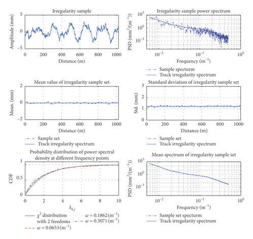
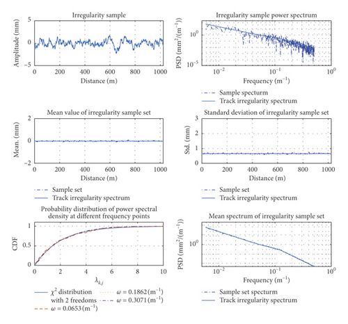
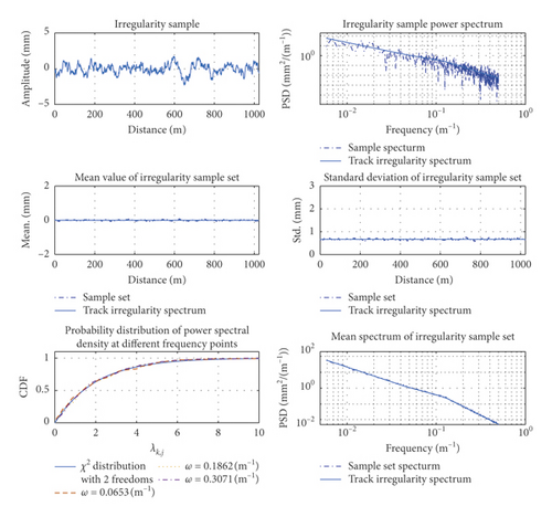
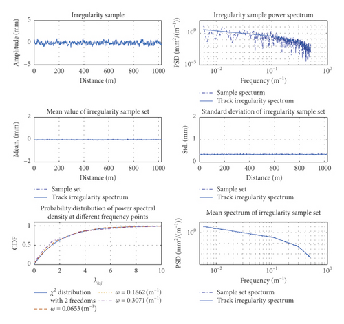
Figure 10 compares the means and standard deviations of the track irregularity in the time domain and the track irregularity spectrum in [31]. The power spectrum of each frequency point in the sample set was tested by χ² distribution with a significance level of α = 0.05 and two degrees of freedom with the Kolmogorov–Smirnov method, verifying the accuracy of the random track irregularities simulated by the present method.

The power spectral density and track irregularity power spectrum derived from a single sample did not accurately estimate the vertical profile, alignment, cross-level, or gage irregularity of the track (Figure 10). However, the mean power spectrum calculated from the sample set of track irregularities favorably agreed with the target spectrum. The maximum difference between the mean vertical profile, alignment, cross-level, and gage irregularity and those obtained from the target spectrum were 0.18 mm, 0.10 mm, 0.07 mm, and 0.08 mm, respectively, with maximum standard deviations of 4.68%, 5.77%, 6.97%, and 6.99%, respectively. In contrast, the maximum deviations in the power spectrum of the sample set were 14.54%, 10.23%, 10.07%, and 9.87%, respectively. In the power spectral densities at different frequencies of the sample set, the vertical profile, alignment, cross-level, and gage irregularity of the track all satisfied the 2-degree-of-freedom χ² distribution (with 98.00%, 96.33%, 98.00%, and 98.33% of the frequency points satisfying the distribution, respectively). Each index of the sample set well agreed with the target spectrum, and only eight random variables were required to extract the indices from the time-domain samples. The method also retained a large number of frequency components. The commonly used trigonometric method, when simulating track random irregularity time-domain samples, requires enough random phase. When there are only 8 random phases, the simulated track random irregularity time-domain samples will have periodic repeatability and cannot be used in the calculation of the vehicle-rail coupled dynamic system. It can be seen that the numerical simulation method in this paper can greatly reduce the number of random variables required to simulate track random irregularity time-domain samples.

2.4. Numerical Solution Method

The track-vehicle coupled dynamic model was solved by an explicit-implicit integration method, with time integral step less than 0.0001 seconds, and the mode number of rail is taken as half the number of rail support points. The displacement and speed of the train and rail at the (n + 1)th moment were computed from the displacement, speed, and acceleration in the nth and (n − 1)th moments. The wheel-rail force was then calculated by the wheel-rail contact model, using the freedoms of the wheelset and rail at the (n + 1)th moment. After forming the wheel-rail load matrix, the fastener model was solved with the rail and slab freedoms, obtaining the wheel-rail load matrix. The vehicle and rail acceleration at the (n + 1)th moment was solved by the vehicle and rail motion equation, and the dynamic response of the slab and base at the (n + 1)th moment under the fastener force load was obtained by the Newmark-β integral method. Finally, the generalized probability density was evolved by the finite difference discretization of the modified Lax–Wendroff scheme [16].

3. Numerical Calculation and Analysis

3.1. Model Verification

3.1.1. Calculation Conditions

The vehicle parameters are shown in Table 2. The analysis was performed on the Chinese high-speed ballastless railway irregularity spectrum, with an irregularity wavelength range of 2–120 m. The vehicle speed was 350 km/h. The track irregularities in the time domain were sampled by the random irregularity numerical simulation method described in Section 2.3. The evaluation indices were the left/right wheel load reduction rates, the left/right wheel derailment coefficients, lateral force of the wheel axis, and the lateral/vertical accelerations of the car body. The calculation results of single and multiple samples were compared and verified.

Table 2. Vehicle dynamics parameters.

Item		Notation	Unit	Value
Car body	Mass	m_c	kg	33.2 × 10³
	Mass moment of inertia about x-axis	Ix_c	kg·m²	1.07568 × 10⁵
	Mass moment of inertia about y-axis	Iy_c	Kg·m²	1.6268 × 10⁶
	Mass moment of inertia about z-axis	Iz_c	kg·m²	1.4027 × 10⁶

Bogie	Mass of bogie	m_t	kg	2.6 × 10³
	Mass moment of inertia about x-axis	Ix_t	kg·m²	2106
	Mass moment of inertia about y-axis	Iy_t	kg·m²	1424
	Mass moment of inertia about z-axis	Iz_t	kg·m²	2600

Wheelset	Mass of wheelset	m_w	kg	1.97 × 10³
	Mass moment of inertia about x-axis	Ix_w	kg·m²	623
	Mass moment of inertia about y-axis	Iy_w	kg·m²	78
	Mass moment of inertia about z-axis	Iz_w	kg·m²	623

Primary suspension system	Longitudinal spring stiffness	k_px	N/m	9.8 × 10⁶
	Lateral spring stiffness	k_py	N/m	9.8 × 10⁶
	Vertical spring stiffness	k_pz	N/m	1.176 × 10⁶
	Longitudinal damping coefficient	c_px	N·s/m	0
	Lateral damping coefficient	c_py	N·s/m	0
	Vertical damping coefficient	c_pz	N·s/m	0.196 × 10³

Second suspension system	Longitudinal spring stiffness	k_sx	N/m	1.784 × 10⁵
	Lateral spring stiffness	k_sy	N/m	1.931 × 10⁵
	Vertical spring stiffness	k_sz	N/m	1.931 × 10⁵
	Longitudinal damping coefficient	c_sx	N·s/m	0
	Lateral damping coefficient	c_sy	N·s/m	5.88 × 10⁴
	Vertical damping coefficient	c_sz	N·s/m	9.8 × 10⁴

Half the transverse distance between vertical primary suspension systems		d_wk	m	1.0
Half the transverse distance between vertical primary suspension system absorber		d_wc	m	1.0
Half the transverse distance between vertical second suspension systems		d_sk	m	1.25
Half the transverse distance between vertical second suspension systems absorber		d_sc	m	1.25
Vertical distance between center of gravity of car body and lateral secondary suspension system		H_cb	m	0.644
Vertical distance between lateral secondary suspension system and center of gravity of bogie		H_bt	m	0.29
Vertical distance between center of gravity of bogie and lateral primary suspension system		H_tw	m	0.08
Half the longitudinal distance between center of rear bogie and center of front bogie		L_c	m	8.75
Half the bogie axle base		L_t	m	1.25

3.1.2. Comparison and Verification of the Single-Sample Calculations

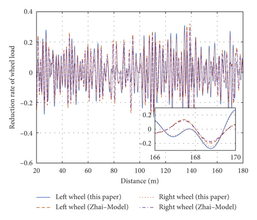
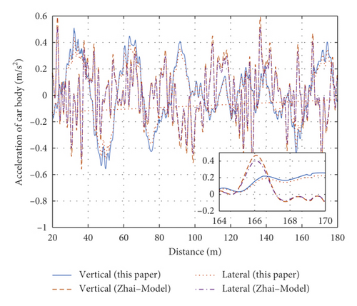
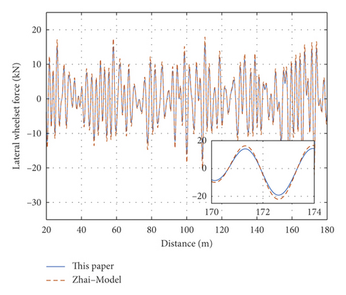
The vehicle-track coupled dynamic model proposed by Zhai and Chen [2, 3] has been widely used, so the dynamic model is verified by comparing the model in this paper with Zhai-model. Figure 11 compares the present calculation results with those of the Zhai-model in the case of a single time-domain sample from the track irregularity data. The calculation parameters and random track irregularity sample were the same in both methods. As the forces on the left and right wheel-rail are unequal, the wheel load reduction rates and derailment coefficients differed between the left and right wheel-rail contacts; see of Figures 11(a) and 11(b) for comparisons of the left and right wheel-rail states, respectively. The maximum differences between the left and right wheel-rail load reduction rates and derailment coefficients were 0.35 and 0.19, respectively. Therefore, the left or right wheel-rail state alone cannot fully reflect the wheel-rail state; both substates must be considered together. Comparing the present calculation model with the Zhai-model, the wheel load reduction rates and derailment coefficients differed by (at most) 8.74% and 7.62%, respectively. Meanwhile, the maximum differences in the vertical and transverse accelerations of the car body were 7.21% and 8.99%, respectively, and the maximum difference in the transverse force of the wheel axle was 6.78%. In summary, the results of the vehicle-track coupled dynamics model and the classical Zhai-model differed by less than 10%, confirming the accuracy of the model developed here.

3.1.3. Comparison and Verification of Multisample Calculation Results

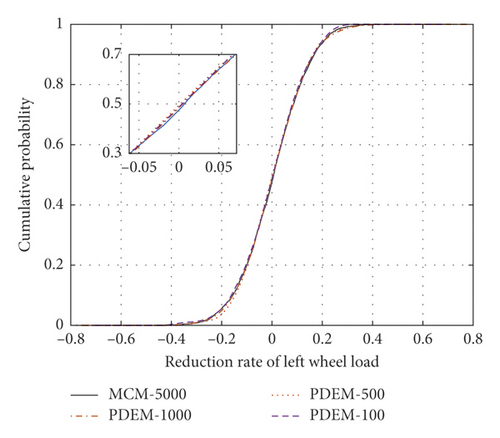
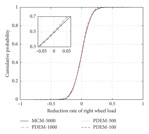
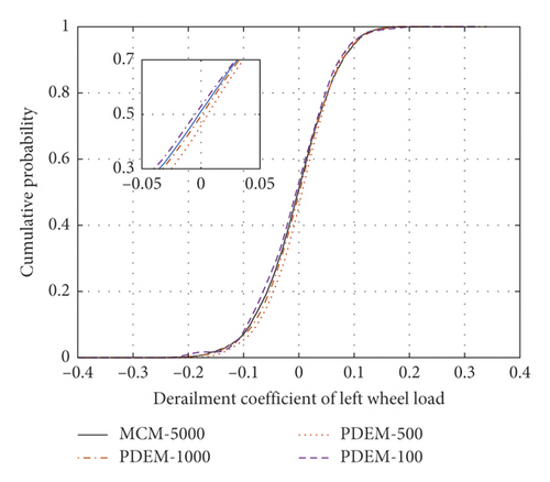
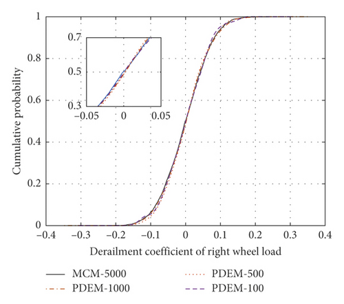
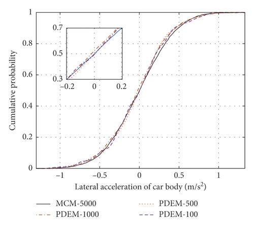
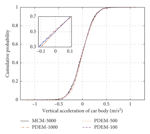
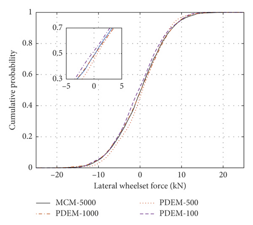
Random variables were selected by the MCM, and the random track irregularity was solved by the trigonometric series method. Five thousand random track irregularity samples were selected for computing the dynamic response of the vehicle-track coupled power system, and the statistical characteristics of each evaluation index were calculated. The probabilistic evolution processes of the indices were then calculated by the developed model, varying the number of samples as 100, 500, and 1000. Figure 12 plots the cumulative probabilities of each index for the different numbers of samples and (for comparison) the cumulative probability in the MCM method with 5000 samples. The sectional cumulative probabilities of the left/right wheel load reduction rates, the left/right wheel derailment coefficients, the vertical/transverse accelerations of the car body, and the lateral force of the wheel axle well agreed with the statistical results of many MCM calculations. However, the developed model greatly reduced the number of required irregularity samples. Figures 12(a) and 12(c) show the sectional cumulative probabilities of the wheel load reduction rates and derailment coefficients, respectively, in the four cases at a fixed distance on the left side (the equivalent plots on the right side are shown in Figures 12(b) and 12(d), respectively). In the single sample analysis, the load reduction rates and derailment coefficients largely differed between the left and right sides, but after selecting 100, 500, or 1000 samples, the cumulative probability distributions of the left and right wheel-rail indices were consistent. The wheel load reduction rates of the developed model with 100, 500, and 1000 samples differed by (at most) 0.068, 0.049, and 0.033, respectively, from those of the MCM with 5000 samples. The corresponding differences between the derailment coefficients computed by the developed method and the MCM were 0.075, 0.040, and 0.029, respectively. Clearly, the developed computational model with multisampling achieves the same computational accuracy as the largely sampled MCM.

3.2. Reliability Analysis of Vehicle Operation Safety

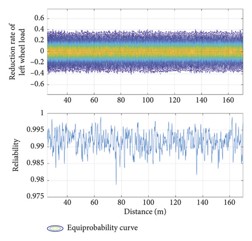
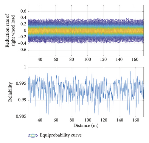
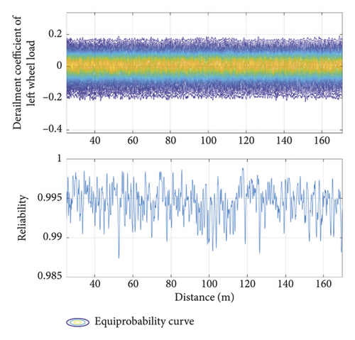
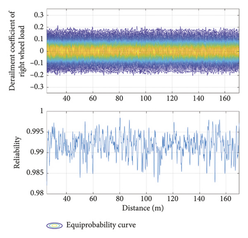
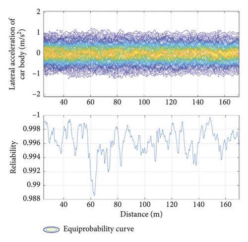
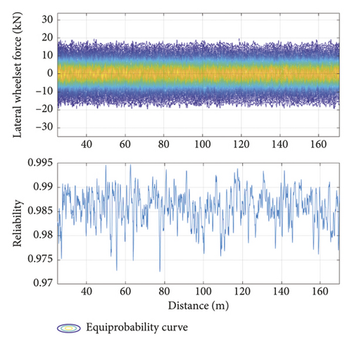
The ballastless track structure in China offers a comfortable riding experience. When a single vehicle is traveling at 350 km/h, its safety evaluation index (calculated by the developed method) meets the requirements of common specifications. As limiting values in the safety evaluation, the wheel load reduction rate was taken as 0.3, the derailment coefficient as 0.15, the lateral and vertical accelerations of the car body as 1.0 m/s² and 0.5 m/s², respectively, and the lateral force as 13 kN. Figure 13 plots the equal-probability and reliability curves of the safety evaluation indices of the running vehicle. The developed model easily evolved the probability of each evaluation index, and all indices spatiotemporally varied with the running mileage. Although the running mileage influenced the reliability of the different indices, it did not affect their equal-probability evolution curves, because the random track irregularity time-domain samples obtained from the track irregularity spectrum is a stationary random process. Table 3 lists the maximum and minimum probabilities of each safety evaluation index under the calculation conditions. The probability values under different limits were quickly calculated, confirming the convenience of the developed model in train operation safety evaluation.

Table 3. Probabilities of limit values of the vehicle-safety evaluation indices.

Evaluating indicator	Reduction rate		Derailment coefficient		Vertical acceleration of car body	Lateral acceleration of car body	Lateral wheelset force
Evaluating indicator	Left	Right	Left	Right	Vertical acceleration of car body	Lateral acceleration of car body	Lateral wheelset force
Min	0.9787	0.9857	0.9874	0.9821	0.9885	0.9853	0.9725
Max	0.9989	0.9988	0.9989	0.9984	0.9997	0.9987	0.9948

3.3. Train Safety Evaluation Indices Limit Value with Different Probabilities

Given a vehicle and track structure with random track irregularities, the calculation results of a single sample cannot obtain the limits of the evaluation indices. In the presence of random irregularities, the limit values can be obtained only with a certain probability. For this purpose, the probabilistic index was introduced, providing a new way of computing the limit values of the indices of vehicle-track coupled dynamics.

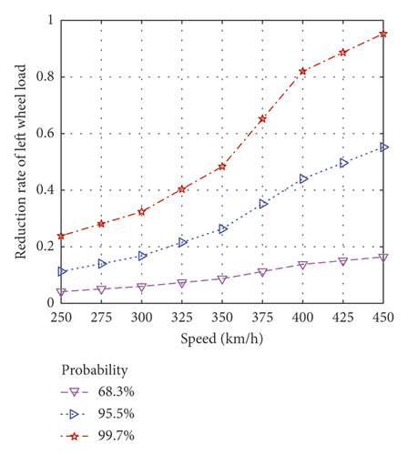
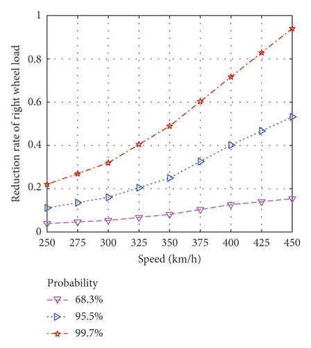
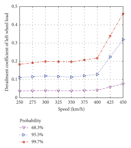
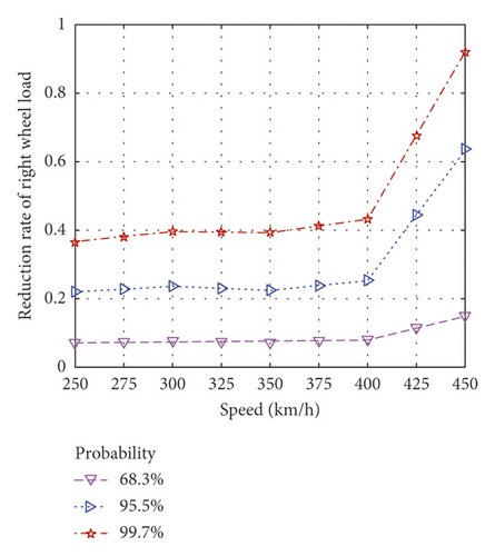
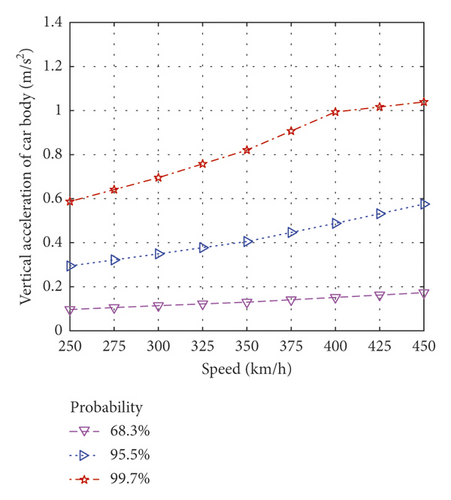
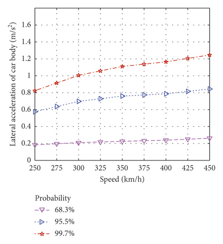
Figure 14 plots the evaluation indices variation curve with vehicle speed computed by the developed model with different index probabilities (1, 2, and 3 times the standard deviation of a normal distribution). At 68.3% probability, the evaluation indices were relatively insensitive to vehicle speed, but at 99.7% probability, they significantly increased with speed. The derailment coefficient was barely affected by vehicle speeds below 400 km/h but rapidly increased at higher speeds (at 450 km/h, the derailment coefficient value at 99.7% probability increased by 123.8%).

4. Conclusions

This paper presents an evaluation model of safe railway operation based on probability theory and a nonlinear vehicle-track coupled power system. The model more accurately captures the force state between the wheel and rail than the linearized vehicle-track coupling dynamic system. The random track irregularities were sampled in the time domain by a stochastic function-spectral representation method, which reduces the required number of samplings. The developed simulation method was verified in comparisons with an established method. The safety of the running vehicles was probabilistically determined by the evaluation indices (derailment coefficient, acceleration of the car body, and the lateral force of the wheel axle). The model results were compared with those of the Zhai-model and the MCM. Next, the vehicle-safety evaluation indices were computed for different probabilities of their limit values. At the lower probability (68.3%), the limiting evaluation indices were little affected by the vehicle speed, but at the highest probability (99.7%), they were significantly increased at higher vehicle speeds. The derailment coefficient deserves special attention when driving at high speed. The developed computational model provides a new research direction for vehicle operation safety evaluation. In future work, the model will be applied to safe railway operation under different conditions, such as different structures, different track or foundation diseases, and different track irregularities.

Conflicts of Interest

The authors declare that they have no conflicts of interest.

Acknowledgments

The research work described in this paper was supported by the High-speed Railway Joint Fund of National Natural Science Foundation of China (grant U1734208), the Major Program of National Natural Science Foundation of China (grant 11790283), the Hunan Provincial Natural Science Foundation of China (grant 2019JJ40384), and the Hunan Provincial Innovation Foundation for Postgraduate (CX2017B058).

Open Research

Data Availability

The analysis result data used to support the findings of this study are included within the article. The calculation data used to support the findings of this study are available from the corresponding author upon request.

References

1 Wu Y.-S., Yang Y.-B., and Yau J.-D., Three-dimensional analysis of train-rail-bridge interaction problems, Vehicle System Dynamics. (2001) 36, no. 1, 1–35, https://doi.org/10.1076/vesd.36.1.1.3567, 2-s2.0-0035405545.
10.1076/vesd.36.1.1.3567
Web of Science® Google Scholar
2 Chen G. and Zhai W. M., A new wheel/rail spatially dynamic coupling model and its verification, Vehicle System Dynamics. (2004) 41, no. 4, 301–322, https://doi.org/10.1080/00423110412331315178, 2-s2.0-2442702736.
10.1080/00423110412331315178
Web of Science® Google Scholar
3 Zhai W. M, Vehicle-Track Coupled Dynamics, 2015, 4th edition, Science Press, Beijing, China.
Google Scholar
4 Lou P. and Zeng Q.-Y., Formulation of equations of motion for a simply supported bridge under a moving railway freight vehicle, Shock and Vibration. (2007) 14, no. 6, 429–446, https://doi.org/10.1155/2007/870830, 2-s2.0-36049036191.
10.1155/2007/870830
Web of Science® Google Scholar
5 Dinh V. N., Kim K. D., and Warnitchai P., Dynamic analysis of three-dimensional bridge-high-speed train interactions using a wheel-rail contact model, Engineering Structures. (2009) 31, no. 12, 3090–3106, https://doi.org/10.1016/j.engstruct.2009.08.015, 2-s2.0-70449712639.
10.1016/j.engstruct.2009.08.015
Web of Science® Google Scholar
6 Zhang N., Xia H., and Guo W. W., Vehicle–bridge interaction analysis under high-speed trains, Journal of Sound and Vibration. (2008) 309, no. 3–5, 407–425, https://doi.org/10.1016/j.jsv.2007.07.064, 2-s2.0-35748938225.
10.1016/j.jsv.2007.07.064
Web of Science® Google Scholar
7 Yang Y. B. and Yau J. D., Vertical and pitching resonance of train cars moving over a series of simple beams, Journal of Sound and Vibration. (2015) 337, 135–149, https://doi.org/10.1016/j.jsv.2014.10.024, 2-s2.0-84916594037.
10.1016/j.jsv.2014.10.024
Web of Science® Google Scholar
8 Chen G., Zhai W. M., and Zuo H., Analysis of the random vibration responses characteristics of the vehicle track coupling system, Journal of Traffic and Transportation Engineering. (2001) 1, no. 1, 13–16.
Google Scholar
9 Xia H., De Roeck G., Zhang H. R., and Zhang N., Dynamic analysis of train-bridge system and its application in steel girder reinforcement, Computers & Structures. (2001) 79, no. 20-21, 1851–1860, https://doi.org/10.1016/s0045-7949(01)00115-8, 2-s2.0-0035416187.
10.1016/S0045-7949(01)00115-8
Web of Science® Google Scholar
10 Au F. T. K., Cheng Y. S., and Cheung Y. K., Effects of random road surface roughness and long-term deflection of prestressed concrete girder and cable-stayed bridges on impact due to moving vehicles, Computers & Structures. (2001) 79, no. 8, 853–872, https://doi.org/10.1016/s0045-7949(00)00180-2, 2-s2.0-0034831520.
10.1016/S0045-7949(00)00180-2
Web of Science® Google Scholar
11 Lu F., Lin J. H., Kennedy D., and Williams F. W., An algorithm to study non-stationary random vibrations of vehicle–bridge systems, Computers & Structures. (2009) 87, no. 3-4, 177–185, https://doi.org/10.1016/j.compstruc.2008.10.004, 2-s2.0-58149479369.
10.1016/j.compstruc.2008.10.004
Web of Science® Google Scholar
12 Zhang Z., Zhang Y., Lin J., Zhao Y., Howson W. P., and Williams F. W., Random vibration of a train traversing a bridge subjected to traveling seismic waves, Engineering Structures. (2011) 33, no. 12, 3546–3558, https://doi.org/10.1016/j.engstruct.2011.07.018, 2-s2.0-80054913560.
10.1016/j.engstruct.2011.07.018
Web of Science® Google Scholar
13 Zeng Z. P., Liu F. S., Lou P., Zhao Y. G., and Peng L., Formulation of three-dimensional equations of motion for train–slab track–bridge interaction system and its application to random vibration analysis, Applied Mathematical Modelling. (2016) 40, no. 11-12, 5891–5929, https://doi.org/10.1016/j.apm.2016.01.020, 2-s2.0-84956860684.
10.1016/j.apm.2016.01.020
Web of Science® Google Scholar
14 Zhang Z. C., Lin J. H., Zhang Y. H., Zhao Y., Howson W. P., and Williams F. W., Non-stationary random vibration analysis for train-bridge systems subjected to horizontal earthquakes, Engineering Structures. (2010) 32, no. 11, 3571–3582, https://doi.org/10.1016/j.engstruct.2010.08.001, 2-s2.0-77957301162.
10.1016/j.engstruct.2010.08.001
Web of Science® Google Scholar
15 Yu Z.-W., Mao J.-F., Guo F.-Q., and Guo W., Non-stationary random vibration analysis of a 3D train-bridge system using the probability density evolution method, Journal of Sound and Vibration. (2016) 366, 173–189, https://doi.org/10.1016/j.jsv.2015.12.002, 2-s2.0-84957430242.
10.1016/j.jsv.2015.12.002
Web of Science® Google Scholar
16 Li J. and Chen J. B., Stochastic Dynamics of Structures, 2009, John Wiley & Sons (Asia) Ptd Ltd, Singapore.
10.1002/9780470824269
Google Scholar
17 Xu L., Zhai W., and Gao J., A probabilistic model for track random irregularities in vehicle/track coupled dynamics, Applied Mathematical Modelling. (2017) 51, 145–158, https://doi.org/10.1016/j.apm.2017.06.027, 2-s2.0-85028732406.
10.1016/j.apm.2017.06.027
Web of Science® Google Scholar
18 Xu L. and Zhai W., A new model for temporal-spatial stochastic analysis of vehicle-track coupled systems, Vehicle System Dynamics. (2017) 55, no. 3, 427–448, https://doi.org/10.1080/00423114.2016.1270456, 2-s2.0-85007371011.
10.1080/00423114.2016.1270456
Web of Science® Google Scholar
19 Rocha J. M., Henriques A. A., and Calçada R., Probabilistic safety assessment of a short span high-speed railway bridge, Engineering Structures. (2014) 71, 99–111, https://doi.org/10.1016/j.engstruct.2014.04.018, 2-s2.0-84899856146.
10.1016/j.engstruct.2014.04.018
Web of Science® Google Scholar
20 Rocha J. M., Henriques A. A., Calçada R., and Rönnquist A., Efficient methodology for the probabilistic safety assessment of high-speed railway bridges, Engineering Structures. (2015) 101, 138–149, https://doi.org/10.1016/j.engstruct.2015.07.020, 2-s2.0-84938090401.
10.1016/j.engstruct.2015.07.020
Web of Science® Google Scholar
21 Rocha J. M., Henriques A. A., and Calçada R., Safety assessment of a short span railway bridge for high-speed traffic using simulation techniques, Engineering Structures. (2012) 40, 141–154, https://doi.org/10.1016/j.engstruct.2012.02.024, 2-s2.0-84860745158.
10.1016/j.engstruct.2012.02.024
Web of Science® Google Scholar
22 Jin Z., Pei S., Li X., and Qiang S., Probabilistic evaluation approach for nonlinear vehicle-bridge dynamic performances, Journal of Sound and Vibration. (2015) 339, 143–156, https://doi.org/10.1016/j.jsv.2014.11.008, 2-s2.0-84919933318.
10.1016/j.jsv.2014.11.008
Web of Science® Google Scholar
23 Cho T., Song M. K., and Lee D. H., Reliability analysis for the uncertainties in vehicle and high-speed railway bridge system based on an improved response surface method for nonlinear limit states, Nonlinear Dynamics. (2010) 59, no. 1-2, 1–17, https://doi.org/10.1007/s11071-009-9521-0, 2-s2.0-77949395951.
10.1007/s11071-009-9521-0
Web of Science® Google Scholar
24 Antolín P., Zhang N., Goicolea J. M., Xia H., Astiz M. Á., and Oliva J., Consideration of nonlinear wheel-rail contact forces for dynamic vehicle-bridge interaction in high-speed railways, Journal of Sound and Vibration. (2013) 332, no. 5, 1231–1251, https://doi.org/10.1016/j.jsv.2012.10.022, 2-s2.0-84871194814.
10.1016/j.jsv.2012.10.022
Web of Science® Google Scholar
25 Li Q., Xu Y. L., Wu D. J., and Chen Z. W., Computer-aided nonlinear vehicle-bridge interaction analysis, Journal of Vibration and Control. (2010) 16, no. 12, 1791–1816, https://doi.org/10.1177/1077546309341603, 2-s2.0-79953662314.
10.1177/1077546309341603
Web of Science® Google Scholar
26 Li J. and Chen J.-B., The probability density evolution method for dynamic response analysis of non-linear stochastic structures, International Journal for Numerical Methods in Engineering. (2006) 65, no. 6, 882–903, https://doi.org/10.1002/nme.1479, 2-s2.0-31644439141.
10.1002/nme.1479
Web of Science® Google Scholar
27 JJ K., On the Rolling Contact of Two Elastic Bodies in the Presence of Dry Friction, 1967, T H Delft, Delft, Netherlands.
Google Scholar
28 Meymand S. Z., Keylin A., and Ahmadian M., A survey of wheel-rail contact models for rail vehicles, Vehicle System Dynamics. (2016) 54, no. 3, 386–428, https://doi.org/10.1080/00423114.2015.1137956, 2-s2.0-84959486547.
10.1080/00423114.2015.1137956
Web of Science® Google Scholar
29 Liang J., Chaudhuri S. R., and Shinozuka M., Simulation of nonstationary stochastic processes by spectral representation, Journal of Engineering Mechanics. (2007) 133, no. 6, 616–627.
10.1061/(ASCE)0733-9399(2007)133:6(616)
Web of Science® Google Scholar
30 Liu Z., Liu W., and Peng Y., Random function based spectral representation of stationary and non-stationary stochastic processes, Probabilistic Engineering Mechanics. (2016) 45, 115–126, https://doi.org/10.1016/j.probengmech.2016.04.004, 2-s2.0-84964334610.
10.1016/j.probengmech.2016.04.004
Web of Science® Google Scholar
31 National Railway Administration, PSD of Ballastless Track Irregularities of High-Speed Railway.(TB/T 3352-2014), 2014, National Railway Administration, Beijing, China.
Google Scholar

Citing Literature

All articles

Stochastic Analysis of Nonlinear Vehicle-Track Coupled Dynamic System and Its Application in Vehicle Operation Safety Evaluation

Abstract

1. Introduction

2. Stochastic Analysis Model of Nonlinear Vehicle-Track Coupled Dynamic System

2.1. Stochastic Analysis Method Based on Generalized Probability Density Evolution Theory

2.1.1. Generalized Probability Density Evolution Theory

2.1.2. Selection of Random Variable Samples and the Probability Assignment

2.2. Vehicle-Track Coupled Dynamics Model

2.2.1. Vehicle Dynamics Model

2.2.2. Dynamic Model of the Track Structure

2.2.3. Wheel-Rail Contact Relation

2.3. Numerical Simulation and Verification of the Random Track Irregularity Model

2.4. Numerical Solution Method

3. Numerical Calculation and Analysis

3.1. Model Verification

3.1.1. Calculation Conditions

3.1.2. Comparison and Verification of the Single-Sample Calculations

3.1.3. Comparison and Verification of Multisample Calculation Results

3.2. Reliability Analysis of Vehicle Operation Safety

3.3. Train Safety Evaluation Indices Limit Value with Different Probabilities

4. Conclusions

Conflicts of Interest

Acknowledgments

Open Research

Data Availability

References

Citing Literature

Figures

References

Information

About Wiley Online Library

Help & Support

Opportunities

Connect with Wiley

Stochastic Analysis of Nonlinear Vehicle-Track Coupled Dynamic System and Its Application in Vehicle Operation Safety Evaluation

Abstract

1. Introduction

2. Stochastic Analysis Model of Nonlinear Vehicle-Track Coupled Dynamic System

2.1. Stochastic Analysis Method Based on Generalized Probability Density Evolution Theory

2.1.1. Generalized Probability Density Evolution Theory

2.1.2. Selection of Random Variable Samples and the Probability Assignment

2.2. Vehicle-Track Coupled Dynamics Model

2.2.1. Vehicle Dynamics Model

2.2.2. Dynamic Model of the Track Structure

2.2.3. Wheel-Rail Contact Relation

2.3. Numerical Simulation and Verification of the Random Track Irregularity Model

2.4. Numerical Solution Method

3. Numerical Calculation and Analysis

3.1. Model Verification

3.1.1. Calculation Conditions

3.1.2. Comparison and Verification of the Single-Sample Calculations

3.1.3. Comparison and Verification of Multisample Calculation Results

3.2. Reliability Analysis of Vehicle Operation Safety

3.3. Train Safety Evaluation Indices Limit Value with Different Probabilities

4. Conclusions

Conflicts of Interest

Acknowledgments

Open Research

Data Availability

References

Citing Literature

Figures

References

Related

Information