Global Sensitivity Analysis of High Speed Shaft Subsystem of a Wind Turbine Drive Train
Abstract
The wind turbine dynamics are complex and critical area of study for the wind industry. Quantification of the effective factors to wind turbine performance is valuable for making improvements to both power performance and turbine health. In this paper, the global sensitivity analysis of validated mathematical model for high speed shaft drive train test rig has been developed in order to evaluate the contribution of systems input parameters to the specified objective functions. The drive train in this study consists of a 3-phase induction motor, flexible shafts, shafts’ coupling, bearing housing, and disk with an eccentric mass. The governing equations were derived by using the Lagrangian formalism and were solved numerically by Newmark method. The variance based global sensitivity indices are introduced to evaluate the contribution of input structural parameters correlated to the objective functions. The conclusion from the current research provides informative beneficial data in terms of design and optimization of a drive train setup and also can provide better understanding of wind turbine drive train system dynamics with respect to different structural parameters, ultimately designing more efficient drive trains. Finally, the proposed global sensitivity analysis (GSA) methodology demonstrates the detectability of faults in different components.
1. Introduction
Nowadays wind turbine industry is growing very fast and wind power has become one of the most cost effective of all renewable energy sources because of environmental concerns and finite resource of fossil fuels [1]. Therefore, it has attracted political and business interest and extensive research is carried out at different universities and institutes [2].
It is very important to reduce the costs of design, manufacturing, and maintenance and optimize the power performance of wind turbines in order to be cost competitive in the current market. A better understanding and consequently improvement of wind turbine drive train dynamics performance could lead to overall cost efficiency in wind turbine operations. This is done by advanced system modelling, identifying the reasons for premature failures and fault diagnoses [3] in different components in drive train of wind turbines. Examples of multibody dynamic analysis to predict the components’ loads in wind turbine drive trains are in [4–6]. Generally, the dynamic performance of wind turbine drive train can be investigated based on different points of view, such as power performance, operational speeds, loads in specific components like coupling and bearings in both healthy and faulty situations, and misalignment parameters [7–14]. Different structural dynamic parameters can directly influence a wind turbine ultimate performance and in terms of loading, high speed shaft components are the most important since the components experience major extreme loads during different regimes, especially in transient one.
The current research deals with mathematical modelling of high speed shaft drive train test rig. A typical wind turbine drive train is composed of a generator as an electrical part with a control set, flexible couplings, a speed-up gearbox, a main shaft, and a wind rotor as an air-operated system [15]. The power from the rotor is transferred through main shaft, gearbox, and high speed shaft to the generator.
We propose the global sensitivity analysis (GSA) as a tool to better investigate wind turbine drive train dynamics, more specifically, high speed shaft drive train models. The aim is to quantify the input structural parameters’ effect to objective functions of the system dynamics (interaction quantification set [16]). From GSA the most influential design parameters on objective functions of wind turbines can be determined, which could ease the optimization process by narrowing down the number of input design parameters.
Methodology of sensitivity analysis is various and it has been used for different applications. Reviews on different GSA methods can be found in [16–20]. Some examples of sensitivity analysis are derivative-based Morris one-at-a-time (OAT) local sensitivity method [21] and Sobol/Saltelli method providing the variance based sensitivity [22, 23], whereas the Sobol/Saltelli variance based sensitivity method provides indices that quantify the relative contribution of each input structural parameter to set of objective functions [22, 23]. In the variance based GSA, input variables are chosen randomly in a proper range. Then, the contribution of input parameter to objective functions is investigated via the sensitivity indices. These sensitivity indices are quantifying the contribution of a random variable to the total variance of the response, which is basis of variance based global sensitivity analysis in [23].
Computational effort when design analysis requires a large set of loading conditions to be evaluated, such as wind turbine drive trains, is very important. As one of the most common methods for GSA, Monte Carlo simulation for these systems is not efficient since it is computationally expensive. On the other hand, GSA within analysis of variance decomposition (ANOVA) or high dimensional model representation (HDMR) theory is suitable method in terms of being cost effective. It decomposes the response function of a high dimensional system into combination of low dimensional system set. This reduces the computational effort. A multiplicative dimensional reduction method (M-DRM) for GSA was proposed by Zhang and Pandey [24] entailing simple representation of GSA indices. The method has proved to be as accurate as Monte Carlo with much less computational effort [22].
Several works have been done within sensitivity analysis of rigid and flexible multibody systems with respect to structural parameters such as mass, moment of inertia, stiffness, and damping values [25–28]. In [29] extended Fourier amplitude sensitivity test method was used and the results of a single turbine and a set of large group of turbines was compared by GSA. Sensitivity analysis to perform a large set of data analysis for a wind farm was reported in [30].
Considering that the faults occur in high speed shaft drive trains, this could be a subject of study [31, 32]. The test rig for high speed shaft drive train as subsystem of wind turbine has been constructed in order to do experimental study and acquire data for validation of developed mathematical model. Another purpose of the test rig is to investigate strategies to detect faults. Early fault detection is important since it can reduce the cost of maintenance drastically.
Ultimately, by introducing faults and defects and different components of high speed shaft drive train, we investigate the detectability of faults and failures within GSA. Such an analysis could lead to fault diagnose in components of wind turbine drive train and prevent failures in early stages.
In the following sections, the proposed mathematical model of high speed shaft drive train test rig with the experimental setup at the lab is presented. Then, input variables and different operational scenarios and objective functions are introduced. Different sources of faults and failures such as defect in the bearing, backlash in the coupling, and torque ripple in the motor are introduced and modelled. Ultimately, the GSA indices for the validated model have been investigated. Results of GSA allow one to understand the priorities in contribution of system parameters for any specific objective function and lead one to focus on the areas of operation that show greatest opportunities for optimization. The outcome of the current research leads to useful information regarding wind turbine drive train dynamics behaviour on different operational scenarios which not only provide possibility to reduce the number of input parameters for optimization and speed up the process, but also give insight to design functional components in proper ranges and in a smarter way. In particular, the main aim of the paper is to apply the GSA for the proposed mathematical model of high speed shaft drive train including aforementioned fault sources. Quantifying the faults effects on the drive train objective functions could be applied as a methodology to contribute to virtual condition monitoring in order to detect and predict faults and prevent failures in early stages in different components of drive trains.
2. High Speed Shaft Drive Train System Test Rig
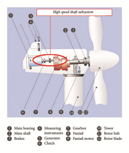
The most common wind turbine is of lateral (horizontal) axis type, which entails main supporting tower upon which sits a nacelle and rotor. Inside the nacelle sits a main shaft supported by bearings on which the rotor hangs. The main shaft is connected to a gearbox, which, in turn, is connected to the generator with control system (Figure 1). The high speed shaft subsystem is one part where faults in bearing are often observed.
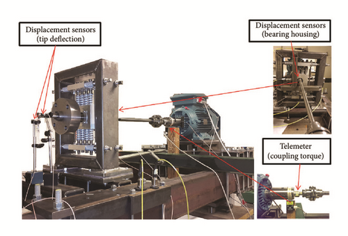
To support experimental and numerical studies of wind turbine drive train dynamics, a scaled down test rig has been built and instrumented as reported in [33, 34]. It entails a motor, rotor disk with shaft, where the rotor shaft is passing through the bearing housing and connected to the motor by a coupling. A small eccentric mass can be added on the rotor disk to give a varying load. The setup of the drive train test rig is represented in Figure 2.
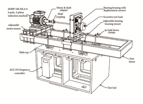
The test rig is driven by ABB motor model M3BP160 MLA 6 (6 pole, 75 kW) with a variable frequency controller (ACS355 from ABB providing speed up to 1000 rpm). In addition, the test rig entails motor shaft adapter, shaft’s coupling, bearing housing with flexible support, a disk on which an eccentric mass can be added, and bedplate on which all the components are mounted.
The data acquisition system is SKF @ptitude Observer; SKF offers under its Windcon 3.0 condition monitoring system. The set of sensors comprise accelerometers and Eddy probes displacement sensors, which detect vibrations in the test rig and deflection at both tip and bearing housing. Additionally, in order to measure the torque in coupling, full bridge strain gauges are put on the motor shaft, and the signal is acquired using a telemeter system (TEL 1-PCM).
In previous works [33, 34], the coupling torque, deflection fields in both lateral and vertical directions in tip, and bearing housing have been measured and used for model validation. To support future studies of defect detection, the objective functions derived in this paper are based on these sensors.
2.1. Mathematical Model of Drive Train System Test Rig
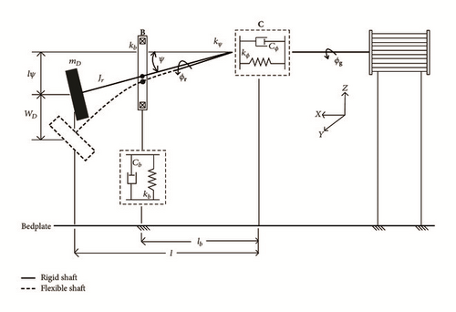
An engineering abstract of the test rig is shown in Figure 3. The mathematical model has been developed based on both rigid and flexible shaft assumption in bending modes, considering that the torsional flexibility is concentrated at coupling. The motor is rigidly attached to the bedplate.
2.1.1. Governing Equations
| Parameter | Symbol | Nominal value (X⋆) | Xmin/X⋆ | Xmax/X⋆ |
|---|---|---|---|---|
| Motor inertia with respect to x axis | Jg | 0.087 kgm2 | 0.5 | 2 |
| Rotor inertia with respect to x axis | Jr | 0.095 kgm2 | 0.5 | 2 |
| Rotor shaft inertia with respect to x axis | Jsh | 0.0003 kgm2 | ||
| Rotor inertia with respect to ψ (minor axis) | Ir | 19.083 kgm2 | 0.5 | 2 |
| Disk inertia with respect to y axis | ID | 18 kgm2 | ||
| Shaft inertia with respect to y axis |
|
0.5 kgm2 | ||
| Disk mass | mD | 14.52 kg | 0.75 | 1.5 |
| Rotor shaft mass | msh | 3.85 kg | ||
| Eccentric mass value mounted in the rotor disk | me | 74.4 gr | 0 | 4 |
| Distance of eccentric mass from center | re | 8 cm | ||
| Rotor shaft and disk mass | mr | 18.35 kg | ||
| Length from coupling to the tip | l | 0.85 m | 0.8 | 1.2 |
| Length from coupling to bearing housing | lb | 0.72 m | 0.8 | 1.2 |
| Length from coupling to CG of disk and rotor shaft | l0 | 0.75 m | ||
| Damping factor | ζd | 0.01 s | ||
| Coupling torsional stiffness | kϕ | 2600 Nm/rad | 0.75 | 5 |
| Coupling bending stiffness | kψ | 56 kNm/rad | 0.75 | 5 |
| Bearing mount lateral and vertical stiffness coefficients |
|
4308 kN/m | 0.75 | 5 |
| Bearing hub bending stiffness |
|
0.1kψ | 0.75 | 5 |
| Coupling torsional damping | Cϕ | 26 kNm/rad | 0.5 | 10 |
| Coupling bending damping | Cψ | 56 kNm s/rad | 0.5 | 10 |
| Bearing mount lateral and vertical damping coefficients | Cb | 4308 kN s/m | 0.5 | 10 |
| Bearing friction damping coefficient | Cbf | 0.0023 Ns/m | 0.8 | 3 |
| Rotor torsional damping coefficient plus bearing friction |
|
0.006 Ns/m | 0.8 | 3 |
| Motor torsional damping coefficient | Cbg | 0.006 Ns/m | 0.5 | 10 |
| Shaft bending stiffness | EI | 7.6699 kNm2 | 0.5 | 10 |
| Angle dependency factor of kb | αb | 1 | 0.8 | 1.5 |
| Torque ripples parameters |
|
10 Nm | 0 | 3 |
| Backlash gap | BL | 0.002 m | 0 | 3 |
| Backlash regularization parameter | σ | 40 | ||
| Bearing torque disturbance zone for defect | ε | 0.1 | ||
| Maximum value of rotational bearing defect torque |
|
30 Nm | 0 | 5 |
| Maximum value of radial bearing defect torque |
|
30 Nm | 0 | 5 |
F is an external load vector and it is a combination of , , and which applies to specific degree of freedom.
corresponds to external forces due to the disturbance of the bearing defects imposed to the system (described in Section 2.2.3). The defect may impose the disturbance torque into bending and torsional degrees of freedom (• = {ψ, ϕr}).
refers to the backlash of the coupling which appears as an internal load in the governing equations. The backlash has a contribution in the potential energy since it is modelled as a spring with gap.
is torque ripples imposed by the motor, a source of faults in drive train dynamics representing electromechanical interaction between components.
2.1.2. Parametrization of the Model
Since the coupling is assumed to be very stiff in torsion (apart from its backlash), the shaft torsional flexibility and coupling play are here added and included in kϕ, and . We introduce ϕr as the rotor (disk plus shaft) angle, such that the shaft twist is represented by where ϕg is the motor shaft angle. Hence, ϕs and ϕD are both replaced by ϕr in the governing equations in Section 2.1.1. We assume that the shaft inertia and coupling are abstracted as Jr = Jsh + JC. Coupling torsional stiffness is represented in a way that includes both shaft and coupling torsional stiffness’s. Similarly, the shaft and coupling damping, and , are represented by Cϕ.
The shaft deflection is parametrized in terms of rigid and flexible contribution to total deflection as w(x) = ψx + wDφ(x), where ψ is the angular deflection at the coupling, wD is the rotor shaft tip deflection due to shaft flexibility, and φ(x) is taken as the shape of the fundamental bending eigenmode as described in [33]. In [33], we developed and validated the mathematical model of high speed shaft drive train test rig considering the shaft flexibility in terms of bending. To obtain a suitable shape function φ(x), the Euler-Bernoulli beam theory is applied [36]. Only radial vibration amplitudes of the beam were considered. The fundamental bending eigenmode based on structural parameters in Table 1 was found at β = 0.8734 and its shape function φ for a shaft rotating at speed Ω = 1000 rpm gives the eigenfrequency at ω⋆ = 109.4608 rad/s. The next eigenmode was found at ω⋆ = 6151 rad/s, which is much higher than relevant excitation frequency. The deflection fields in two locations, namely, tip (x = l) and bearing hub (x = lb), are assessed within the aforementioned assumptions. Thus, the tip radial deflection would be ψl + wDφ(l), and the bearing housing radial deflection becomes ψlb + wDφ(lb). The displacements in vertical and lateral directions become mirrored by rotational angle ϕr. Note that we simplify the deflection field in the bearing hub. For more realistic model, shaft prebending and relative motion of inner ring with respect to the bearing hub frame must be considered.
To conclude, the vector of generalized coordinate is defined as .
2.2. Faults Modelling in the Drive Train
2.2.1. Electromechanical Modelling of the Motor: Motor Torque with Ripple
Considering that wind turbine drive train contains both mechanical and electrical components, it is of important concern to have a model which studies electromechanical interactions. In induction motors, many kinds of excitation occur such as electromagnetic forces exist, that is, unbalanced magnetic pull. Torsional vibration of drive train system could lead to significant fluctuation of motor speed. Such oscillation of the angular speed superimposed on the average motor angular speed causes severe oscillation of electric currents in motor windings [37]. In this section, we model torque ripple as source of this fluctuations in motor speed.
2.2.2. Backlash Modelling of the Coupling
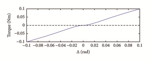
2.2.3. Modelling of Defects in Rolling Elements (Bearing): Disturbance Torque from Bearing Inner Ring
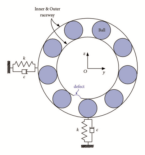
Bearing fault diagnosis is important in condition monitoring of any rotating machine. Early fault detection is one of the concerns within the wind turbine system modelling. To this end, we need to model source of faults in the bearing. Dynamic modelling and vibration response simulation of rolling bearings with surface defects is a common assumption within fault modelling. When bearing balls roll over defects, shock pulses with high frequency are generated with excessive vibration leading the whole system to failure. This characteristic impulse-response signal is detected by the vibration monitor. An inner raceway rotates with shaft’s rotation and goes through the loaded zone of bearing every rotation. This mechanism shows that the vibration of inner raceway with defect is modulated by the shaft rotation [39–41].
Here we propose a simple modelling of surface defect for bearing which imposes a disturbance torque in certain angles in the inner raceway connected to the rotor shaft (similar to when a ball passes from the defects and causes a excitation to the system). Figure 5 shows the external torque imposed in radial and rotational directions. As part of external forces, is defined based on impulse factor ε and maximum torque as shown in Figure 5(a).
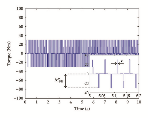
Proper value for maximum disturbance is Nm. ε(=0.1) is the angular length of active contact zone, where the defect is assumed (Figure 5).
2.2.4. Uneven Mounting Stiffness
2.3. Numerical Values of Parameters in the High Speed Shaft Drive Train Test Rig
Table 1 represents the parameters and their numerical values assumed in the mathematical model:
The damping coefficients are chosen as proportional to respective stiffness coefficient: C•≐ζdk•, where • = {ϕ, ψ, b}.
The value of Cbf which represents the bearing friction damping has been defined from SKF manual handbook [42].
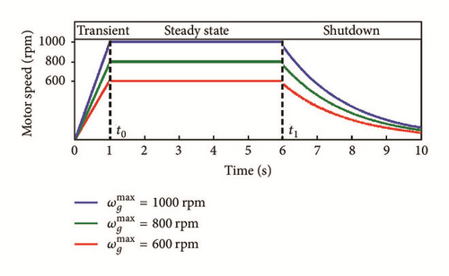
2.4. Operational Scenarios
- (i)
Transient: a torque is applied to reach the preset speed.
- (ii)
Steady state: it is where the structure is under almost constant speed control.
- (iii)
Shutdown: in this regime there is no torque imposed to the system, and it is left to slow down to stop.
Note that the corresponding motor speeds ( rpm) correspond to the specific frequency in the frequency controller ( Hz, resp.).
2.5. System Model Response for the Nominal Values
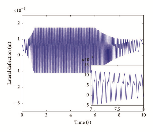
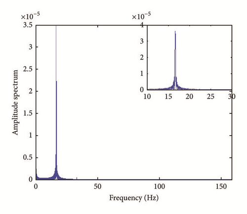
Here, we present the simulation response of the mathematical model based on structural parameters nominal values represented in Table 1. The displacement fields in both lateral and vertical direction with their FFT have been presented.
The deflection fields include three different operational scenarios based on Figure 6 with steady state of sec and shutdown starting at t = 6 sec. The tip deflection fields in both vertical and lateral directions are presented with zoom in steady state ( sec) and shutdown ( sec) in Figure 7.
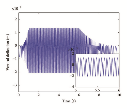
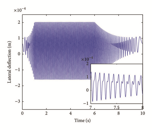
The bearing housing deflection fields in both vertical and lateral directions are presented with zoom in steady state ( sec) and shutdown ( sec) are shown in Figure 8.

The frequency response functions of the tip deflection in both vertical and lateral directions are presented with zoom on the dominant frequency in Figure 9.
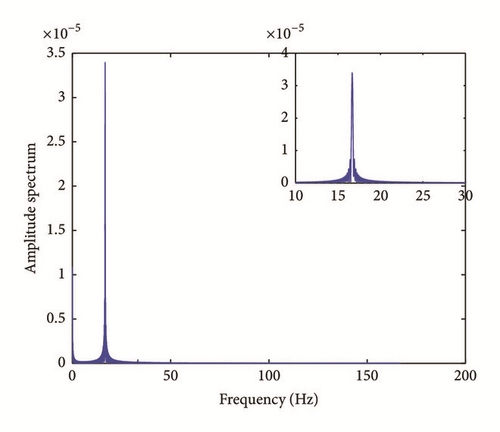
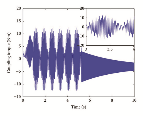
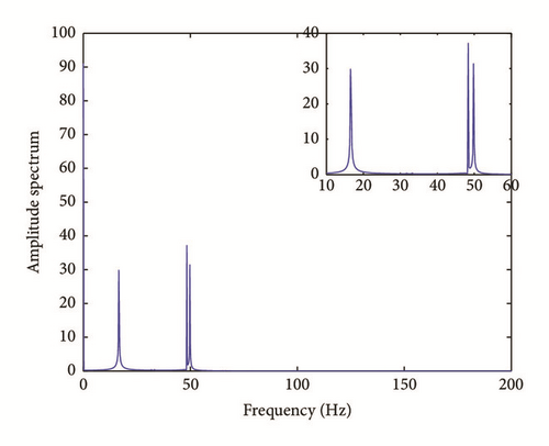
The coupling torque with its frequency response is presented here in Figure 10.
The equations of motion have been solved using Newmark numerical procedure method implemented in Matlab software. In order to satisfy the convergence criteria, the proper time step has been chosen as Δt = 10−4.
3. Objective Functions
In this section we introduce the set of objective functions. The introduced objective functions are assessed in order to evaluate the dynamic performance of the developed high speed shaft models.
(i) Tip Deflection in Both Vertical and Lateral Directions in Steady State and Shutdown Regimes . The RMS values of the tip deflection in both lateral and vertical in two operational scenarios (steady state and shutdown) (RMS(Ystd), RMS(Zstd) and RMS(YSD), RMS(ZSD), resp.) are obtained within the mathematical model and the sensitivity indices based on the structural inputs have been defined for these objective functions.
(ii) Bearing Hub Deflection in Both Vertical and Lateral Directions in Steady State and Shutdown Regimes . RMS value of the bearing housing bending in both lateral and vertical directions in two operational scenarios (steady state and shutdown) (, and , , resp.) is obtained within the mathematical model and the sensitivity indices based on the structural inputs have been defined for these objective functions. A model of gearbox is required to consist of shaft and bearing housing stiffness, which allows interaction between housing and the internal components to be investigated.
(iii) Frequency Response of the Tip Deflection in Lateral and Vertical Directions in Steady State and Shutdown . These are the desired objective function representations: FFT(Ystd), FFT(Zstd) and FFT(YSD), FFT(ZSD), respectively. The modal sensitivity analysis allows one to recognize the eigenfrequency response to design parameters changes. It can also help for the better identification of important dynamic properties.
(iv) Coupling Torque in Different Operational Scenarios Transient, Steady State, and Shutdown Cases . In order to determine the influence of the design parameters in torsional vibration model, RMS values of the coupling torque in different operational scenarios transient, steady state, and shutdown cases are investigated as objective functions (RMS(CTtr), RMS(CTstd), and RMS(CTSD), resp.). The coupling torque is defines as Mϕ = kϕΔ.
Coupling torque in transient regime is very important to measure and quantify the parameters which have the most effect, since the component experiences the most severe loadings due to this regime nature. By shutting down the motor, there is not any load imposed by motor side and the range of the coupling torque is decreased from steady state value to zero in short period of time.
(v) The First and Second Peaks in FFT Diagram of Coupling Torque in Steady State . There are several picks in the coupling torque frequency response, of which the most dominant one is of interest to study, and investigating the most influential parameter would give valuable conclusion form the vibrational point of view. Studying the torsional model, we came up with a conclusion that some peaks in FFT are related to the ripple due to motor. Quantifying those peaks would give the contribution of the fault source to the objective function, which is very valuable information in terms of optimization.
(vi) The Peak in FFT Diagram of Coupling Torque in Shutdown Regime . During shutdown we expect that only torsional eignefrequency of the structure plays the role in FFT.
4. Global Sensitivity Analysis of High Speed Shaft Test Rig
The efficiency and applicability of global sensitivity analysis is already proven by some mathematical and mechanical examples [24]. The aim here is to apply this method to the high speed shaft drive train dynamics with respect to the structural parameters.
4.1. Theoretical Concept of Variance Based Sensitivity Analysis
Each of the objective functions in Section 3 can be seen as a function of the test rig structural parameters, represented as vector of n variables, X = [X1, X2, …, Xn] T. We have adopted the variance based sensitivity indices developed by Saltelli et al. [43] and mainly founded on the previous work of the Russian mathematician Zhang and Pandey [22]. These methods are defined as global sensitivity analysis (GSA), since the set of sensitivity indices are calculated considering the entire range of variations in parameters, compared to OAT (once at a time) or differential approaches [44].
In case Xi’s are not uniformly distributed, it is possible to define a probability function for random variables X1, X2, …, Xs and adjust (12) and (13) accordingly [22].
4.1.1. Multiplicative Dimensional Reduction Method (M-DRM): To Compute the Simplified Sensitivity Indices
The primary sensitivity index, Si, gives an indication of how strong the direct influence of Xi is on OF without any interactions with other variables. The total sensitivity index, , gives an indication of the total influence of Xi on OF from its own direct effects along with its interaction with other variables [49, 50].
The differences between the primary effect and the total effect then give an indication of how important the interactions of Xi are with other variables in influencing OF. If the main effect is small, whereas the total effect is large, then Xi does influence OF but only through interactive effects with other system inputs.
The introduced sensitivity indices accuracy depends on number of integration points used that can be determined via a convergence study [24, 51].
4.2. System Input Parameters Used in GSA
The nominal values of the input parameters as well as the range of parameters variation are given in Table 1. X⋆ is chosen as cut point (see Section 4.1.1).
5. Results from GSA of High Speed Shaft (HSS) Model
In this section, the global sensitivity analysis of the developed mathematical models corresponding to high speed shaft drive train system has been presented. Both torsional and bending models are examined under three different operational scenarios with different motor speeds in steady state ( Hz).
The analysis presented here focuses on the response characteristics particular to chosen objective functions. It is expected that the operational scenarios will influence the dynamics and structural response to different input variables.
5.0.1 Convergence Study. The number of function evaluations using M-DRM method is NX × N. For specific set of input variables and on each operational scenario, all objective functions are evaluated at the same time by a single time integration of the model. In order to achieve an acceptable approximation of the sensitivity analysis indices using the M-DRM method, it is important to assess the convergence of the results by increasing number of Gaussian quadrature integration abscissas denoted by N in (18).
The convergence study shows that for a nonlinear system such as high speed shaft drive train with system input parameters prescribed in Section 5, sufficient level of accuracy for the sensitivity analysis can be obtained with 21 × 20 = 420 (NX = 21 design parameters and N = 20 integration abscissas) function evaluations. This is one of the most prominent aspects of the global sensitivity analysis using this approach, which could reduce the computational effort drastically.
5.1. GSA of Drive Train High Speed (HSS) Shaft Subsystem Model
In this section we apply GSA to the total model which comprises bending and torsional parameters all together. The input parameters are defined in (20).
For the model containing all bending and torsional parameters, the primary and total sensitivity indices are as shown in Figure 11.
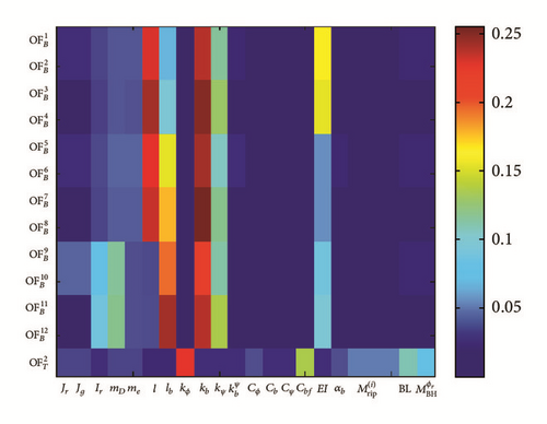
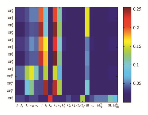
It can be concluded from this that the torsional input parameters (coupling torsional stiffness kϕ and bearing damping due to friction Cbf and motor torque ripples , backlash parameter BL, and bearing impact disturbance ) do not have significant influence to the bending objective functions (). The same conclusion could be made based on the bending input parameters (coupling bending stiffness kψ and bearing mounting stiffness kb and shaft bending stiffness EI) which do not seem to have major effect on torsional objective function ().
Based on this analysis, we conclude that the torsional and bending response of the model can be analysed separately, which allows for substantially simpler analysis, which will discussed next.
5.2. HSS Bending Model
After separating the two models, we analyse the sensitivity of HSS within the frame of bending model based on bending objective functions such as deflection field in bearing hub and tip in both lateral and vertical directions and the corresponding frequency domains.
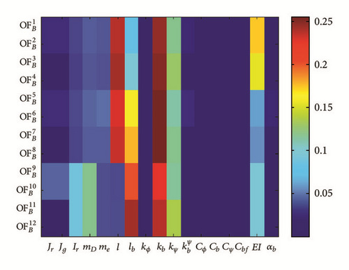
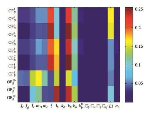
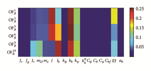
It was shown that within these 3 different motor frequencies, the contribution of the input parameters is not changing drastically. The obtained results of GSA are presented in Figure 12. The results indicates that the most influential structural parameters which have the major effect to the objective functions are coupling bending stiffness kψ and bearing mounting stiffness kb, shaft bending stiffness EI, and bearing hub and tip locations lb, l. Also, the damping parameters do not have significant effect on both primary and total sensitivity indices.
More detailed analysis of the results based on each objective functions and influence of the input parameters is presented as follows.
(i) Tip Deflection in Vertical and Lateral Directions in Steady State and Shutdown Scenarios . It is illustrated that the coupling bending stiffness kψ and bearing hub mounting stiffness kb are the most dominant influential parameters, respectively.
It could be seen from Figure 12 that the shaft bending stiffness EI has more influence in tip deflection field compared to the other objective function. This is somehow logical since the first bending mode shape is higher in tip (x = l) compared to bearing hub (x = lb) [33].
Moreover, the geometric locations of bearing hub and tip (lb, l) are influential parameters in terms of deflection field in both bearing hub and tip.
(ii) Bearing Hub Deflection in Vertical and Lateral Directions in Steady State and Shutdown Scenarios . In bearing deflection field the influence of lb is more than l. In tip deflection field the influence of l is more than lb.
The bearing bending stiffness does not have a major effect to the system objective functions.
It could be seen that the angle dependency of the bearing stiffness αb is not having a major effect to all of objective functions, since the realistic range for αb is small.
(iii) Frequency Response of the Tip Deflection in Vertical and Lateral Directions in Steady State and Shutdown Scenarios . The influences of stiffness parameters kψ and kb and EI and lb and also inertia parameters Ir, mD, and me are the most dominant parameters, respectively. This tells that aforementioned parameters are the most important ones in terms of frequency response of the tip deflection.
Among the mass inertia parameters, Ir, me, and mD affect most of the bending objective functions.
It could be also seen form Figure 12 that the damping input parameters have the least influences on both primary and total sensitivity indices.
To sum up the conclusion related to the GSA of HSS subsystem within the frame of bending model, kb and kψ and EI and Ir and mD and me have the major effects on both primary and total sensitivity indices.
However, according to the sensitivity analysis results, rest of parameters stated in the system modelling do not have a remarkable effect on the mentioned objective functions. Such information would be particularly useful in attenuating the number of design parameters for optimization applications of wind turbine drive trains setups which leads to cost efficient simulations.
5.3. Bending Model with Bearing Defect: Detection of Faults in Inner Ring
Here, we study the bearing defect influence to the objective functions. The aim is to investigate the sensitivity indices with respect to the bearing defect parameter imposing a radial load to the bearing housing and seek its effect to the bearing deflection and loads.
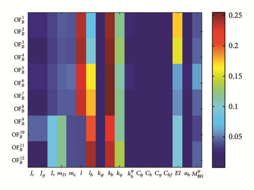
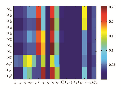
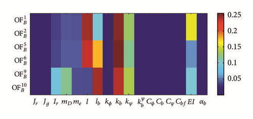
It is hypothesized that if the sensitivity index with respect to parameter is comparable to other sensitivities in certain OF, we can expect that a sensor measuring this OF is able to detect defects of size related to the magnitude of . The obtained results on GSA with bearing defect are presented in Figure 13 and summarized below.
- (i)
Deflection fields in vertical and lateral directions in steady state and shutdown scenarios for the tip () and bearing hub (), respectively: in Figure 13, comparing sensitivity indices for objective functions tip and bearing hub deflections ( versus ), the influence of the bearing defect in bearing hub is more than the tip. This is due to direct influence of the defect in the bearing by imposing the defect torque, which means that the bearing may experience more damage by introducing a defect in the inner ring.
- (ii)
Frequency response of the tip deflection in steady state () and shutdown () scenarios: in FFT of tip deflection, bearing defect has shown different influence compared to the healthy case (no defect). This means that the frequency response of structure in both healthy and faulty conditions is different and by studying FFT of system response and investigating their sensitivity indices, we could detect some faults sources in specific components.
5.4. HSS Torsional Model
The torsional model has been studied based on the faults sources introduced in the previous sections. Backlash effects on coupling creating nonlinearities to the system structure, motor torque ripple with specific peaks in the frequency domain, and bearing defect disturbance torque imposing on the rotor angular direction are applied within system modelling. In order to optimize the design and upgrade the structural performance, the system response must be studied based on these assumptions and compared with the healthy conditions. This gives a better insight to understand the faults sources and could facilitate the way to prevent the failures in drive train by creating structures which are less sensitive with respect to these faults sources. This could be studied within GSA by investigating and optimizing the sensitivity indices.
5.4.1. Torsion Vibration Model of Drive Train Test Rig with Backlash
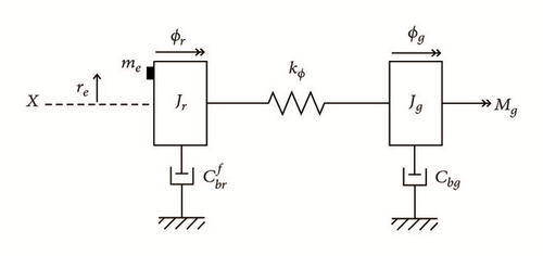
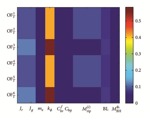
Upon considering only the torsional response of the test rig, the complete model in Section 2.1 is reduced, a lumped torsion vibration model. An engineering abstract of the model is depicted in Figure 14 and entails two inertias, disk Jr and generator rotor Jg, respectively. Each of these inertias is supported by bearings. The shaft and coupling flexibility is lumped together and represented by a torsion spring. Due to gravity and eccentric mass, there will be an external torque Mr(=meregcosϕr) acting on the disk, and the induced electrical torque from the motor Mg acts on the generator rotor.
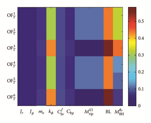
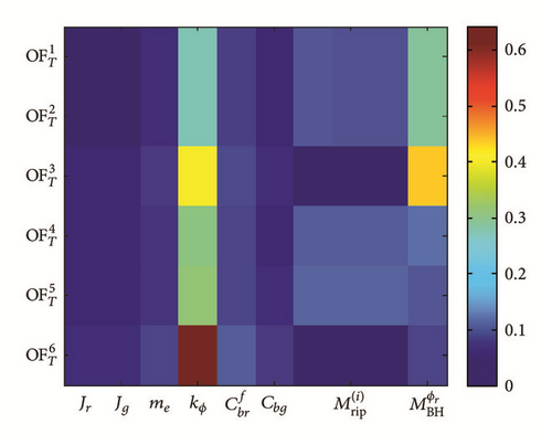
Based on the results (see Figure 15), it could be demonstrated that the most influential input parameters to the torsional objective functions are coupling torsional stiffness kϕ and backlash in coupling BL, motor torque ripples , and bearing defect parameter . Also, the structural damping of the rotor and bearing friction coefficient has some effects to both primary and total sensitivity indices. The effects of damping coefficient (except the bearing damping) and rotor and motor mass inertia values (Jr and Jg) are not significant compared to the other aforementioned parameters. In total sensitivity , also eccentric mass has shown some impact which is expectable since it imposes an external torque to the structure.
More detailed analysis of the results based on each objective functions and influence of the input parameters is stated as follows.
(i) Coupling Torque in Transient and Steady State Regimes . The coupling torque has strong sensitivity in terms of torque ripple parameters arising from the motor. This tells the significance of motor ripple assumption in drive trains as one type of fault source.
(ii) Coupling Torque and Its FFT in Shutdown Regime . It is clear that in shutdown regime there is no any torque ripple imposed by the motor, of which objective functions and sensitivity indices for torque ripples are identically zero.
In FFT, coupling torque influence is more than steady state case, since there is no ripple imposed by the motor. Also eccentric mass has some contribution especially in total sensitivity index.
(iii) Frequency Response of the Coupling Torque in Steady State Regime . In FFT of the coupling torque in steady state regime, the most dominant parameter is kϕ. Then the backlash and motor torque ripples have significant contribution. This tells that in vibration analysis it is very important to identify the vibration faults sources namely here backlash and ripple, which may affect the system structure in a severe way.
(iv) Bearing Defect Maximum Value . By increasing the bearing defect maximum torque (Figure 5), we could investigate its contribution to the sensitivity indices. The aim is to define the minimum value of defect parameter such that the sensitivity indices related to this parameter would be larger than a specific value ( Nm). This methodology contributes to detect, predict, and prevent the faults and failures in bearings.
Summing up the results of GSA for torsional model, we could state that the most influential parameters are kϕ and faults sources BL and and also Cbf, respectively.
For disturbance torque coming from bearing housing , we notice that its influence is more in total sensitivity index rather than primary one. This means that influence is more when the other parameters are changed. The same conclusion could be made for ripple parameters .
5.4.2. Torsional Model with No Backlash
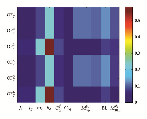
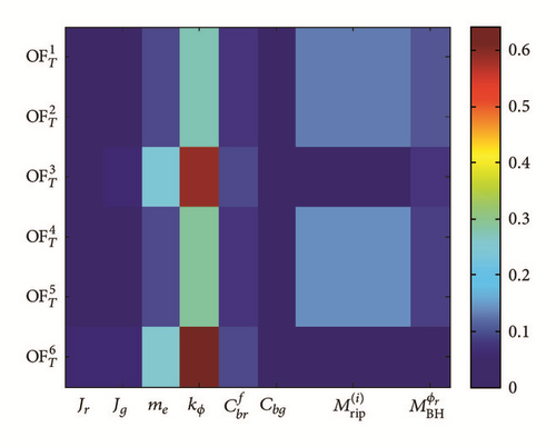
In order to emphasize into the bearing fault detection, we study the system structure response based on no backlash (Figure 16). Then, we investigate the influence of the input parameters to the objective functions in case when the shaft coupling has a backlash.
- (i)
The bearing defect (quantified in terms of ) could be detected easier in case where no backlash compared to with backlash (more contribution sensitivity indices especially the primary one). This is very important conclusion and means that, in the systems with a couple of sources of faults, the detectability of each fault may not be easy and it get more complex by introducing more complex system and assuming more faults.
- (ii)
The influence of bearing defect in the FFT for first peak and the second peaks is small, though recognizable. This draws the same conclusion for the bending model with defect, which tells that some specific peaks in the FFT correspond to the system structural faults.
5.5. Special Cases: Resonance Investigation
The operating speed ranges in wind turbines and system excitation frequency have a wide range. The system may encounter resonances leading to severe vibration and affect the normal operation of the machine. Thus, the drive train dynamics must be studied with more focus in excitation ranges.
- (i)
By selecting those randomized variables which based on them the eigenfrequency of the structure is near to specific value (50 Hz), the sensitivity of eigenfrequency variables takes the most contribution. This is expectable since in the resonance points the system influential parameters are only the ones which the eigenfrequency of the system is based on them.
- (ii)
In optimum case, where the randomized values are identical to the bending and torsional eigenfrequencies, we expect that only the input parameters have influence that they are in the eigenfrequency definition.

6. Conclusion and Outlook
The global sensitivity analysis for both torsional and bending models of high speed shaft drive train test rig with respect to its structural parameters has been carried out using M-DRM method.
The current study showed the feasibility and efficiency of the M-DRM for global sensitivity analysis of nonlinear dynamical system (high speed shaft drive train), which provided the results in a computationally efficient framework. The M-DRM applied here revealed practical significant results which can reduce the number of input design parameters for optimization of wind turbine drive train systems.
By comparing the sensitivity of objective functions with respect to different input structural parameters, a better understanding of drive train system dynamics is obtained. Vertical and lateral deflections in bearing housing and tip, coupling torque in 3 different operational scenarios, FFT of these functions, have been introduced as the objective functions to represent the test rig dynamic performance. To reflect the effect of operational scenarios, the aforementioned outputs have been evaluated within transient, steady state, and shutdown cases in 3 different motor speeds. The effect of the fundamental structural parameters on the dynamic response of the HSS drive train test rig has been recognized. By comparing the sensitivity indices of corresponding objective functions, a better understanding of drive train system dynamics is obtained.
- (i)
GSA for complex systems is computationally expensive by using ordinary algorithms like Monte Carlo. Nevertheless, M-DRM method has been successfully applied to high speed shaft drive train model and provided physically reasonable results in an efficient computational framework.
- (ii)
For considered HSS drive train system model, the estimated primary and total sensitivity indices coincide, revealing no variance interaction effects between the input parameters within different operational scenarios. Also there is a direct correspondence between Si and , which means that the higher order effects are negligible.
- (iii)
Deflection fields in both tip and bearing hub are mostly sensitive with respect to bearing mounting stiffness kb and coupling bending stiffness kψ and geometric parameters l, lb and shaft bending stiffness EI.
- (iv)
Coupling torque mostly in all regimes is influenced mainly by coupling torsional stiffness kϕ, coupling backlash BL, and motor torque ripples , respectively. This means that the proposed faults sources may lead to drastic contributions in components loads. In this research we have quantified these contributions.
- (v)
Dynamic modelling and vibration responses simulation are important for fault mechanism studies to provide proofs for defect detection and fault diagnose. The most significant demonstration in the presented research is the applicability of GSA towards defect detection and faults diagnose in functional components of drive train. The results suggest that, from sensitivity indices, detectability of some faults such as bearing defect could be analysed. This analysis illustrates the applicability of the GSA method for advancing modern condition monitoring systems for bearings.
The global sensitivity analysis provided a useful method to deeply understand some aspects of the initial structural parameters to the dynamic outputs. At this stage, a preliminary assessment of the key parameters has been performed. Moreover, fault modelling in functional components such as motor ripples, bearing defects, coupling backlash, and their detectability within GSA has been investigated. This facilitates understanding the faults sources and their effect to other functional components, which leads to better design and optimize drive trains more efficiently with less failure.
- (i)
Apply GSA for real wind turbine structural parameters such that we first propose to apply the same analysis for NREL 5 MW wind turbine and investigate GSA sensitivity indices.
- (ii)
Carry out dimensional analysis and upscaling of the test rig and apply GSA for Pi Buckingham theory: the aim is to prescribe system structure based on minimal number of dimensionless parameters, which could lead to upscale the structure and predict the real wind turbine behaviours.
- (iii)
Apply wind turbine aerodynamic loads as an external load to the rotor (Mr): in order to get more realistic response of the system, considering the stochastic nature of wind loads, it would be interesting to study the current model based on realistic calculated aerodynamic loads extracted from FAST software.
- (iv)
Study the bearing modelling in more advanced and detailed approach: the bearing defects here have been modelled by introducing an radial excitation to certain DOFs imposed on inner ring of the bearing. For future work, it is important to consider also ball mass inertia and outer ring dynamics [40, 41].
- (v)
Model the electromechanical interaction of wind turbine drive train: since wind turbine contains both mechanical and electrical components, to have better understanding of drive train dynamics, the study must be done within this interaction.
Conflicts of Interest
The authors declare that they have no conflicts of interest.
Acknowledgments
This project is financed through the Swedish Wind Power Technology Centre (SWPTC). SWPTC is a research centre for design of wind turbines. The purpose of the centre is to support Swedish industry with knowledge of design techniques as well as maintenance in the field of wind power. The centre is funded by the Swedish Energy Agency and Chalmers University of Technology as well as academic and industrial partners. In particular, a donation of motors and frequency converters by ABB CR, WindCon3.0 condition monitoring system, and set of sensors by SKF is gratefully acknowledged. Besides, the authors would like to thank Jan Möller for his contribution in the laboratory.


