The Comparison of Grey System and the Verhulst Model for Rainfall and Water in Dam Prediction
Abstract
A time series of data of rainfall in Thailand between the years 2005 and 2015 was employed to predict possible future rainfall based on Julong Deng’s grey systems theory and the grey Verhulst model to see which model can predict more accurately with uncertain and limited data. Firstly, the rainfall data were arranged to display the overall patterns of rainfall volume along with its frequency as well as the temperature during Thailand’s rainy seasons. This makes it possible to see the cycle of rainfall, which is too long for people to intuitively understand the nature of precipitation. One puzzling phenomenon that has made rainfall forecast elusive is the unpredictability of the haphazard nature of rainfall in Thailand. A more precise prediction would certainly result in a better control of water volume in rivers and dams for fruitful agricultural business and adequate human consumption. This can also prevent the flooding that can devastate the economy and transportation of the whole country and also tremendously improve the future water management policy in many ways. This effective prediction could also be employed elsewhere around the globe for similar benefits. Hence, the grey systems theory and the grey Verhulst model are juxtaposed to determine a better prediction possible.
1. Introduction
Water is extremely important to Thailand’s agriculture as well as people largely because the country’s physical terrain is rather flat and consequently appropriate for agriculture while the densely populated cities require ample supply of water for daily use and consumption. Such needs for water would not have been a serious problem if there had been adequate reservoirs and means to conserve rain water for later uses. What has exacerbated the problems is the haphazard nature of precipitation patterns during the rainy seasons. Such uncertainty results in prolonged droughts and severe floods. Fortunately, to relieve his people’s suffering from having too much or too little water, the late King Bhumibol Adulyadej initiated various Royal projects of water resource development and management. Some examples are water resources development at Huay Hong Krai National Park, Doi Saket, and Huay Jo Reservoir, Chiang Mai; drainage projects from lowland and swamp areas of Bacho, Bacho, Narathiwat; building water reservoirs in strategic regions of Thailand, for instance Pa Sak River Dam; and flood relief projects in Lopburi and Saraburi. The king had also invented a method to resolve water shortage problems in other ways such as the cloud seeding procedure for artificial rains [1].
With technological and theoretical advances in science and mathematics during this decade, however, the outlook of rainfall prediction has been improved. Beginning in 1982, Professor Julong Deng’s grey systems theory [2] has attracted worldwide attention of researchers and has been utilized in diversified fields of study such as natural science, engineering science, and many others [3]. Grey systems theory focuses mainly on systems that have partially known and unknown information. Other solutions similar to grey systems were initiated through technological progression. Solutions to uncertain systems have become a challenge for further development in any associated fields. However, one possible means can be provided by different variations of grey systems theory [4]. GM(1,1) model is an important model in grey models family. The procedure to construct the GM(1,1) model, however, is neither a differential equation nor a difference equation. It is an approximate model which has dual characteristics of both differential and difference equations. However, it is inevitable for the approximate model to yield some errors in practical applications. To increase the prediction accuracy of GM(1,1) model, researchers concentrate on the improvements of GM(1,1) model [5] in three main aspects, one of which is the adjustments of grey derivative. Although types of improvements of grey models may increase the precision in some practical way, there are still some existing gaps to improve the precision of any prediction with the use of GM(1,1) model. A novel approach to optimize the initial condition in time response function for general grey prediction model involving the GM(1,1) is proposed, and the grey Verhulst model is opted as its special cases. The optimization approach comprised the detailed item in the time response function from the original GM(1,1) model and the nth item of X(1) [6]. The corresponding weighted coefficients of the two parts, forming the initial condition in new optimization method, are derived from minimizing errors in the summation of square in terms of time response function [7]. The combination of newly initial conditions of fuzzy set and rough set can now express the principle of new information priority which is fully emphasized on in grey systems theory. Hence, the full utilization of new pieces of information can be as follows.
2. The Process Data Sequence of Grey Model
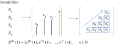
From the matrix above, the optimized data for computing from group data are selected initially. The group of rainfall and temperature data points that are close (or similar) to each other are clustered to identify such groupings (or clusters), using Mathlab [8].
Mathlab graphic [8] representation below indicates that the ranges of temperature that rainfall occurs lie between approximately 25 and 35 degrees Celsius. It is interesting to note that most of the rainfall clusters between 30 and 35 degrees Celsius, while there is very little rainfall (outliers) between the temperatures of 25 and 30 degrees Celsius. As a result, it is possible to forecast the quantity of rainfall using Mathlab to graphically represent when and in what condition the rainfall occurs [7, 9, 10]. (Figure 1). In other words, the density of the clusters is a very good indicator of overflowing, adequate, or insufficient water from the rainfall, the information of which can be very helpful to water management, especially in the prevention of droughts or floods in Thailand.

3. Methodology
- (1)
Grey numbers with only a lower bound: This kind of grey number ⊗ is written as ⊗ ∈ [, ∞] or ⊗ (), where a stands for the definite, known lower bound of the grey number ⊗. The interval [, ∞] is referred to as the field of ⊗.
- (2)
Grey numbers with only an upper bound: This kind of grey number ⊗ is written as ⊗ ∈ (−∞,] or ⊗ (), where a stands for the definite, known upper bound of ⊗.
- (3)
Interval grey numbers: This kind of grey number ⊗ has both a lower and an upper bound , written as ⊗ ∈ [, ].
Another fundamental rainfall and water in dam of uncertain systems was the inaccuracy naturally existing in the available data. After choosing the quantity to reflect the GM(1,1) of the system concerned, one needs to determine the factors that influence the behavior of the system. If a quantitative analysis is considered, one needs to process the chosen actual data and the effective factors using sequence operators so that the available data are converted to their relevant nondimensional values of roughly equal magnitudes.
The calculation of GM(1,1) is performed as follows:
4. Verhulst Model
The GM(1,1) model is suitable for sequences that show an obvious exponential pattern and can be used to describe monotonic changes [6]. As for nonmonotonic wavelike development sequences or saturated sigmoid sequences, one can consider establishing GM(2,1) and Verhulst models, and then, the comparison between two different grey prediction models of rainfall and water in dam is made.
The second calculation of the effect of the same data comparison and prediction of the result is changed in the approach of f2(c). The improved values of the smooth curve and square function are continuously increased.
We can obtain the estimate of c so that it minimizes the f1(c) or f2(c).
The optimized grey systems model, the optimization of initial condition for general form of grey prediction model, is considered, and some optimal forecasting of rainfall is derived. This section takes a look at the optimization of mean values and model parameters for the general grey prediction model defined.
The solution of the parameter vector can be obtained by using the least square method.
And find :
The basic idea for adjusting and optimizing regional structure of agriculturalists is to select and optimize the development of the dominant cultivators so that they can effectively perform the task of farming using the principle of “Sufficient Economy” according to the late King Rama 9th of Thailand [13] (Table 1).
| Rank | Precision level | Meaning of forecast |
|---|---|---|
| A | Less than 0.1 | High accurate predictability |
| B | 0.1-0.2 | Good predictability |
| C | 0.2−0.5 | Reasonable predictability |
| D | More than 0.5 | Inaccurate predictability |
5. Numerical
-
Step 1. GM (1,1)
6. Results and Discussion
The different results of the water and rainfall forecasting are value x(0)(i) – transformed to absolute value. As a result, the error of each prediction can be measured. The error is in the form of a percentage for a more accurate measurement, while the levels of tolerance do not exceed 5%.
6.1. Optimization of Mean Values of Water and Rainfall of Prediction Models
The optimized grey systems model and the adjustment of precision grey model for the general form of grey prediction model are employed, and some optimal forecasting of rainfall is derived. This section takes a look at the optimization of mean values and model parameters (MAPE) for the general grey prediction [14] model as defined by (27), (30), and (31).
In Table 2, the discrepancy of relative errors between GM(1,1) and GVM is obvious. And the relative errors of GVM indicate that it is a more effective predictor than GM(1,1) (Figure 2).
| Year | Value of rainfall (mm) | GM(1,1) | Grey Verhulst model | Comparison | |||
|---|---|---|---|---|---|---|---|
| Forecasted | Relative error | Forecasted | Relative error | GM | GVM | ||
| 2005 | 1,391.13 | 1,391.13000 | 0.000000 | 1,391.13000 | 0.0000000 | A | A |
| 2006 | 1,294.38 | 1160.639126 | 0.103320811 | 1268.777091 | 0.019780056 | B | A |
| 2007 | 1,127.55 | 1090.839652 | 0.032557623 | 1103.82589 | 0.021040407 | A | A∗ |
| 2008 | 1,273.20 | 1403.074098 | 0.102006046 | 1252.684884 | 0.016113035 | B | A |
| 2009 | 1,055.85 | 1040.43307 | 0.014601439 | 1032.535472 | 0.022081288 | A | A∗ |
| 2010 | 1,279.60 | 1481.163528 | 0.157520731 | 1260.451645 | 0.014964329 | B | A |
| 2011 | 1,622.40 | 1599.647364 | 0.014024061 | 1598.961774 | 0.014446639 | A | A∗ |
| 2012 | 1,184.70 | 819.8702634 | 0.307951158 | 1154.556153 | 0.025444288 | C | A |
| 2013 | 1,416.22 | 1488.707888 | 0.051184059 | 1394.610077 | 0.015258875 | A | A∗ |
| 2014 | 1,142.98 | 984.3991677 | 0.138743313 | 1116.887803 | 0.022828218 | B | A |
| 2015 | 1,082.38 | 1197.139254 | 0.106024921 | 1061.569763 | 0.019226368 | B | A |
| MAPE | 0.102793416 | MAPE | 0.01911835 | B | A | ||
- Source: Thailand Meteorological Department.

From the actual data above, the grey Verhulst model’s forecasting power of rainfall data of each year is better than the GM(1,1) model because most of the relative errors are as low as or lower than those forecasted by the GM(1,1). However, such comparison cannot give the whole picture of the water remaining in the dams for use by agriculturalists. The accuracy of the calculation is approximately less than 5% (MAPE = 0.04249 in Table 3). And here, the two models, GM(1,1) and Verhulst model, are employed to compare the accuracy of prediction once again.
| Year | Water in dam (MCM) | GM(1,1) | Grey Verhulst model | Comparison | |||
|---|---|---|---|---|---|---|---|
| Forecasted | Relative error | Forecasted | Relative error | Precise model | |||
| 2005 | 438 | 438.0000 | 0.0000 | 438.0000 | 0.0000 | A | A∗ |
| 2006 | 1627 | 1697.094408 | 0.043081996 | 1619.2925 | 0.004737247 | A | A∗ |
| 2007 | 1917 | 1999.758645 | 0.043170915 | 1886.765149 | 0.015771962 | A | A∗ |
| 2008 | 1690 | 1762.845604 | 0.043103908 | 1653.978051 | 0.021314763 | A | A∗ |
| 2009 | 882 | 919.5604189 | 0.042585509 | 850.516227 | 0.035695888 | A | A∗ |
| 2010 | 2274 | 2372.348758 | 0.043249234 | 2258.133293 | 0.006977444 | A | A∗ |
| 2011 | 2145 | 2237.715356 | 0.043223942 | 2101.732322 | 0.020171412 | A | A∗ |
| 2012 | 510 | 531.3152594 | 0.041794626 | 469.3646272 | 0.079677202 | A∗ | A |
| 2013 | 1469 | 1532.194582 | 0.043018776 | 1459.992114 | 0.006131985 | A | A∗ |
| 2014 | 634 | 660.7303126 | 0.042161376 | 606.8758104 | 0.042782633 | A∗ | A |
| 2015 | 230 | 239.08772 | 0.039511826 | 218.7315064 | 0.04899345 | A∗ | A |
| MAPE | 0.042490211 | MAPE | 0.028225398 | A | A∗ | ||
- Source: The Thai Royal Irrigation Department.
This section takes a look at the ordering of the forecasting power, from A to D, while A is the best and D is the worst according to MAPE, respectively. A < A∗, which means that although A is highly accurate in terms of predictability, A∗ is even a more accurate indicator of predictability.
In Table 3, the point of using grey forecasting will be to predict the next year′s water volume in Thailand as well as rainfall. During the forecasting process, as compared to Table 2, the grey forecasting model should be operated in accordance with the principle of keeping the same dimension rainfall in dam data series (Table 6) [15]. And it appears that the relative errors of GVM indicate that this model is a more effective predictor. So, the importance about the 2012 result difference predicted from data in Tables 2 and 3 is that it has a high error in GVM bar in a point on the graphs. The major causes of annual precipitation and the number of dams are strongly correlated by the observation of the floods in late 2011 to early 2012 (Figure 3) [15].

Finally, by using MAPE to pinpoint the minute differences in the predictive power of both models, it can be clearly seen that Table 3 shows a better picture of the superior power of the Verhulst model to predict the water remaining in the dam for actual use because the MAPE rankings predicted by grey Verhulst model are much better in most cases.
7. Conclusion
Agriculture depends on rainfalls and the quantity of water available for farmers. Good planning will result in proper and adequate use of water for agriculturalists. However, the unpredictability of the quantity of rainfalls each year is affected by many factors unknown to agriculturalists, and by using MAPE and the comparison between grey GM(1,1) and grey Verhulst model, it is possible to predict the total rainfalls in Thailand. By applying MAPE again, the calculation of the water remaining in the dam for use turned out to be even more accurate, judging from the MAPE value of each data range. This can provide a way to deal with unpredictability in the best manner. Therefore, the grey model systems have been proposed to deal with uncertainty of data in the most systematic way.
This paper demonstrates how the grey systems theory has been employed to deal with the prediction problems with incomplete or unknown information with large samples. It is also an attempt to bridge the gap between the immeasurably great works of the late King Rama 9th of Thailand [13], who had devoted a large part of his entire life to improve the welfare of his citizens, especially agriculturalists through various means. In conclusion, the performance of the grey Verhulst model is more superior to the GM(1,1) model because it has the benefits of simplicity for application and a higher forecasting precision [16]. Therefore, we suggest the use of the grey Verhulst model to predict the volume of water in dams of Thailand and other countries for water management planning for agriculture and other similar purposes.
Conflicts of Interest
The authors declare that they have no conflicts of interest.
Appendix
- (1)
x(0)(k) + az(1)(k) = b
- (2)
x(0)(k) = β − αx(1)(k − 1) and
- (3)
x(0)(k) = (β − αx(0)(1))e−a(k−2).
-
Step 1. Compute the accumulation generation of X(0) as follows:
-
Step 2. Check the quasismoothness of X(0).
-
Step 3. Determine whether or not it complies with the law of quasiexponentiality.
From Table 4, we can find c. We will see the differences in the c-values of GM and GVM are enhanced. Because the data are of goodness-of-fit statistics, when considering the MAPE, and with this, we can see the classification accuracy of each model using the grey Verhulst model. All of GVM’s c-values are lower than GM(1,1), which indicate more accurate prediction.
| Value c | GM(1,1) | GVM |
|---|---|---|
| C1 | 31.93143 | 7.403989 |
| C2 | 136.9025 | 7.360478 |
| C3 | 10.75728 | 0.134105 |
| C4 | 212.3465 | 0.613811 |
| C5 | 17.5156 | 0.01174 |
| C6 | 374.3047 | 0.058171 |
| C7 | 81.64682 | 0.002942 |
| C8 | 161.9077 | 0.001353 |
| C9 | 127.0117 | 0.000246 |
| C10 | 192.5966 | 8.65E − 05 |
From Table 5, both the quasismoothness and quasiexponentiality are satisfied (Table 6).
| k | Quasismoothness | Quasiexponential |
|---|---|---|
| 1 | 1.074746211 | 0.930452222 |
| 2 | 1.147957962 | 0.871112038 |
| 3 | 0.885603205 | 1.129173873 |
| 4 | 1.205853104 | 0.829288407 |
| 5 | 0.825140669 | 1.211914571 |
| 6 | 0.788708087 | 1.267896218 |
| 7 | 1.369460623 | 0.730214497 |
| 8 | 0.836522574 | 1.195425002 |
| 9 | 1.239059301 | 0.807063874 |
| 10 | 1.055987731 | 0.9469807 |
| Dam | 2003 | 2004 | 2005 | 2006 | 2007 | 2008 | 2009 | 2010 | 2011 | 2012 | 2013 | 2014 | 2015 |
|---|---|---|---|---|---|---|---|---|---|---|---|---|---|
| Unit: sMCM | |||||||||||||
| Northern | |||||||||||||
| Bhumibol | 7,852.81 | 6,000.10 | 7,250.70 | 6,755.00 | 6,839.70 | 5,101.74 | 7,874.10 | 9,156.24 | 4,298.49 | 3,930.61 | 2,560.90 | ||
| Sirikit | 6,759.33 | 6,261.00 | 6,321.70 | 6,266.00 | 6,720.40 | 3,918.83 | 9,498.29 | 8,158.97 | 4,292.41 | 4,306.35 | 4,490.16 | ||
| Mae Ngad | 331.31 | 403.50 | 319.40 | 350.00 | 120.20 | 202.23 | 458.75 | 276.70 | 192.37 | 222.01 | 176.79 | ||
| Kiu Lom | 562.22 | 980.70 | 474.00 | 473.00 | 543.31 | 730.76 | 1,500.42 | 665.61 | 554.78 | 490.20 | 263.42 | ||
| Mae Kuang | 213.25 | 188.83 | 122.00 | 266.00 | 238.10 | 133.00 | 164.80 | 99.08 | 319.08 | 272.41 | 157.76 | 167.61 | 68.76 |
| Kiu kho mha | 160.80 | 205.66 | 474.24 | 66.51 | 144.07 | 231.60 | 87.19 | ||||||
| Kwai Noi | 920.70 | 1,196.38 | 2,899.93 | 1,211.39 | 1,533.37 | 923.51 | 765.03 | ||||||
| Sum | 15,718.92 | 188.83 | 122.00 | 13,911.30 | 14,603.90 | 13,977.00 | 15,469.91 | 11,454.68 | 23,024.81 | 19,807.84 | 11,173.24 | 10,271.88 | 8,412.25 |
| Northeastern | |||||||||||||
| Lam Pao | 1,818.72 | 1,893.90 | 2,490.20 | 2,236.00 | 1,988.90 | 2,227.28 | 2,825.88 | 2,206.08 | 240.23 | 1,231.64 | 1,246.90 | ||
| Lam Ta Khong | 198.19 | 230.10 | 71.00 | 283.20 | 269.50 | 205.00 | 164.10 | 259.28 | 439.99 | 329.92 | 146.65 | 285.15 | 158.47 |
| Lam Pa Peung | 201.76 | 179.41 | 47.00 | 156.00 | 150.70 | 180.00 | 159.00 | 319.11 | 216.35 | 165.04 | 215.21 | 164.99 | 54.41 |
| Nam Oun | 421.42 | 217.23 | 377.50 | 242.50 | 403.00 | 391.50 | 161.53 | 423.82 | 417.70 | 224.82 | 312.06 | 218.29 | |
| Ubonrat | 2,481.98 | 948.00 | 2,254.60 | 3,898.00 | 2,048.40 | 3,172.75 | 4,641.91 | 1,735.34 | 1,249.84 | 1,144.49 | 470.38 | ||
| Sirinthorn | 856.07 | 1,477.20 | 1,669.30 | 1,348.00 | 1,741.40 | 579.27 | 1,321.89 | 889.31 | 1,430.55 | 2,004.35 | 453.84 | ||
| Chulaporn | 165.37 | 108.29 | 50.00 | 139.30 | 118.50 | 174.00 | 160.30 | 235.23 | 259.22 | 142.50 | 107.68 | 123.18 | 85.86 |
| Huai Luang | 110.15 | 132.58 | 54.00 | 102.20 | 107.30 | 123.00 | 160.40 | 76.71 | 254.74 | 94.49 | 35.35 | 77.78 | 36.54 |
| Lam Nangrong | 10.76 | 17.34 | 13.00 | 25.70 | 28.40 | 15.00 | 24.30 | 20.50 | 23.63 | 40.28 | 121.24 | 39.91 | 20.92 |
| Nam Moon | 86.39 | 102.53 | 32.00 | 76.60 | 119.30 | 71.00 | 123.00 | 60.00 | 170.00 | 127.39 | 58.48 | 96.62 | 41.43 |
| Nam Pung | 77.25 | 133.37 | 200.00 | 106.40 | 123.00 | 121.00 | 87.60 | 81.70 | 169.68 | 118.79 | 73.06 | 46.21 | 48.37 |
| Lam Seah Lam | 187.41 | 116.02 | 103.00 | 144.00 | 192.70 | 168.00 | 238.40 | 157.85 | 234.58 | 334.28 | 167.75 | 263.70 | 123.90 |
| Sum | 6,615.47 | 1,236.87 | 570.00 | 5,730.00 | 7,766.00 | 8,942.00 | 7,287.30 | 7,351.21 | 10,981.69 | 6,601.13 | 4,070.85 | 5,790.09 | 2,959.31 |
| Central | |||||||||||||
| Pa Sak | 1,711.81 | 3,085.10 | 2,383.70 | 2,727.00 | 2,099.10 | 3,260.88 | 4,469.46 | 1,145.71 | 2,109.78 | 1,151.13 | 803.61 | ||
| Kasiew | 247.57 | 73.00 | 273.40 | 497.00 | 501.00 | 287.90 | 593.74 | 414.58 | 320.01 | 156.92 | 321.57 | 125.95 | |
| Tapsaloaw | 131.47 | 42.28 | 38.00 | 117.50 | 174.90 | 246.00 | 164.50 | 172.87 | 183.83 | 110.61 | 149.10 | 66.23 | 27.47 |
| Sum | 2,090.85 | 42.28 | 111.00 | 3,476.00 | 3,055.60 | 3,474.00 | 2,551.50 | 4,027.49 | 5,067.87 | 1,576.33 | 2,415.80 | 1,538.93 | 957.03 |
| Western | |||||||||||||
| Srinakarin | 5,623.07 | 4,372.40 | 4,913.30 | 4,360.00 | 5,396.40 | 4,946.70 | 5,635.98 | 6,153.07 | 5,794.98 | 4,788.58 | 2,104.83 | ||
| Vajiralongkorm | 7,303.40 | 5,360.90 | 6,155.00 | 6,222.60 | 4,417.41 | 4,336.38 | 6,774.76 | 5,639.64 | 5,070.31 | 3,927.87 | |||
| Sum | 5,623.07 | — | — | 11,675.80 | 10,274.20 | 10,515.00 | 11,619.00 | 9,364.11 | 9,972.36 | 12,927.83 | 11,434.62 | 9,858.89 | 6,032.70 |
| Eastern | |||||||||||||
| Bang Pha | 21.80 | 26.18 | 37.00 | 33.00 | 27.90 | 33.00 | 43.00 | 40.31 | 51.92 | 42.93 | 46.65 | 61.07 | 63.79 |
| Nhongpralhai | 177.18 | 159.04 | 243.00 | 144.90 | 182.30 | 171.00 | 228.10 | 194.17 | 317.52 | 191.56 | 385.50 | 254.11 | 51.42 |
| Praprong | 153.00 | 207.90 | 202.20 | 161.00 | 262.90 | 268.96 | 361.11 | 326.46 | 364.69 | 330.98 | 180.53 | ||
| Sriyad | 383.20 | 175.20 | 377.00 | 275.80 | 220.43 | 659.50 | 298.69 | 292.04 | 248.92 | 191.59 | |||
| Sum | 198.98 | 185.22 | 165.10 | 204.00 | 230.00 | 190.40 | 207.63 | 331.69 | 228.91 | 216.34 | 104.09 | 176.58 | |
| Southern | 433.00 | 934.10 | 791.60 | 972.00 | 1,000.20 | 931.50 | 1,721.74 | 1,088.55 | 1,305.21 | 999.16 | 663.91 | ||
| Kaeng Krachan | 866.21 | ||||||||||||
| Pranburi | 743.79 | 1,551.40 | 1,137.60 | 703.00 | 1,017.40 | 583.63 | 626.84 | 876.21 | 918.13 | 978.62 | 664.47 | ||
| Rajjaprabha | 1,815.42 | 245.00 | 987.80 | 347.00 | 390.00 | 482.60 | 315.54 | 218.86 | 252.19 | 487.60 | 387.06 | 264.41 | |
| Banglang | 913.01 | 2,897.30 | 2,427.80 | 2,035.00 | 2,598.40 | 2,645.61 | 2,879.14 | 3,710.79 | 2,185.59 | 2,621.14 | 1,820.36 | ||
| Bangwas | 2,041.90 | 1,608.40 | 2,129.00 | 1,672.60 | 1,691.68 | 1,993.04 | 1,710.19 | 1,300.41 | 1,427.89 | 1,858.87 | |||
| Sum | 4,338.43 | — | 245.00 | 7,478.40 | 5,520.80 | 5,257.00 | 5,771.00 | 5,236.46 | 5,717.88 | 6,549.38 | 4,891.73 | 5,414.71 | 4,608.11 |
| Total | 34,585.72 | 1,653.20 | 1,481.00 | 43,205.60 | 42,012.10 | 43,137.00 | 43,698.91 | 38,365.45 | 56,486.35 | 48,551.07 | 35,291.46 | 33,873.67 | 23,633.31 |
- Source: Royal Irrigation Department of Thailand. The values given in italics are uncertain.
Using Relation Information. A search of the Chinese Data Base of Scholarly Periodicals (CNKI) shows that, from 1990 to 2008, the number of scholarly publications with one of the keywords “fuzzy mathematics,” “grey systems,” and “rough set” also shows an uptrending development. See Tables 7–9 for more details [6].
| Time | 1990 | 1991 | 1992 | 1993 | 1994 | 1995 | 1996 | 1997 | 1998 | 1999 |
| Number of papers | 345 | 373 | 401 | 346 | 543 | 575 | 574 | 551 | 514 | 530 |
| Time | 2000 | 2001 | 2002 | 2003 | 2004 | 2005 | 2006 | 2006 | 2007 | 2008 |
| Number of papers | 605 | 583 | 598 | 714 | 720 | 799 | 908 | 1006 | 933 | 11618 |
| Time | 1990 | 1991 | 1992 | 1993 | 1994 | 1995 | 1996 | 1997 | 1998 | 1999 |
| Number of papers | 149 | 181 | 195 | 203 | 517 | 477 | 481 | 483 | 448 | 456 |
| Time | 2000 | 2001 | 2002 | 2003 | 2004 | 2005 | 2006 | 2006 | 2007 | 2008 |
| Number of papers | 418 | 435 | 512 | 556 | 550 | 576 | 652 | 730 | 762 | 8781 |
| Time | 1990 | 1991 | 1992 | 1993 | 1994 | 1995 | 1996 | 1997 | 1998 | 1999 |
| Number of papers | 0 | 0 | 0 | 0 | 0 | 0 | 1 | 1 | 9 | 19 |
| Time | 2000 | 2001 | 2002 | 2003 | 2004 | 2005 | 2006 | 2006 | 2007 | 2008 |
| Number of papers | 50 | 102 | 142 | 267 | 412 | 553 | 710 | 779 | 919 | 3964 |
- (1)
The mathematical foundation of the uncertain systems theories;
- (2)
The modeling of uncertain systems and computational schemes, including various uncertain system modeling, modeling combined with other relevant methods, and related computational methods; and
- (3)
The wide-range applications of uncertain systems theories in natural and social sciences.