Reliability Analysis to a Satellite-Equipped Harmonic Gear Drive Subjected to Multisource Data and Imbalanced Information

1. Introduction and Motivation

Possessing the advantages of scalability, tractability, and modularity [1], the multilevel hierarchical structure is widely adopted in the design of complex engineering systems. Such systems are deployed to meet highly sophisticated and advanced requirements on functionalities and performance for their applications in mission-critical industries, for example, infrastructure, manufacturing aviation, and high-level national security. Their failure in use would result in devastating consequences. A multilevel hierarchical engineering system may consist of multiple subsystems that are composed of multiple lower-level subsystems or components. In this article, a component, a subsystem, or the whole system is referred to as an “element.” These elements are interconnected and interact with each other, jointly contributing to the functionality of the whole system.

Recent years witness the development of effective approaches (e.g., stochastic process approach and universal generating function approach) in the multilevel system reliability modeling, as summarized in [2]. For a multilevel hierarchical system, one critical issue is to accurately model and analyze the reliability for the whole system under an information imbalance scenario. To illustrate, the available information of a hierarchical system is taken into consideration. The bottom-level elements mostly are standard components with high volume of production and deployment, which yield either readily accessible or easily obtainable reliability information. However, since the experiments for a system as a whole are often costly and time-consuming, accumulated knowledge at the system level is limited and reliability information is often scarce or even absent for top-level elements. Usually, the information of bottom-level components is more easily obtained than that of the top system-level components, which produces the so-called information imbalance scenario [3]. Under such circumstance, it is desirable to aggregate the lower-level information to compensate higher-level information inadequacy for a better reliability estimation at the system level. Frequentist approaches are mathematically cumbersome in information aggregation [3]. Alternatively, Bayesian approaches provide satisfactory and flexible ways to aggregate the available multilevel reliability information [4]. For example, Johnson et al. [5] present a “full-Bayesian approach” for integrating all the reliability information related to a system. This approach resolves the upward and downward propagation problem by simultaneously modeling the complete set of system parameters. Hamada et al. [6] generalize their procedure to the fault tree quantification. Li et al. [7] propose a semiparametric modeling approach for hierarchical systems with multilevel information aggregation. Benefiting from the successful application of the Markov chain Monte Carlo (MCMC) methods in Bayesian inference, the choice of prior distribution is not limited within conjugate distributions and the modelling to multitype data has been significantly extended. Recent works include Li et al. [8], Pan and Yontay [9], Guo et al. [10] are well summarized in [11–18].

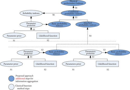
Another critical issue in reliability modeling and assessment field for the multilevel complex system is the difficulty in dealing with heterogeneous data sets. Subjected to costly and time-consuming reliability tests, the available datasets of many higher-level elements of the multilevel system are often restricted to attribute data (e.g., pass/fail data). By contrast, the collected information or data is abundant for lower-level components and exhibits as more informative forms (e.g., the failure time data or degradation data). Methods for system reliability analysis with lifetime or degradation data have been put forward by Huang et al. [19], Wang et al. [20], and Ye et al. [21]. But most of the aforementioned studies are focused on one type of data, while little attention has been paid on a scenario of mixed multisource data, and limited exceptions are the work proposed by [22–25]. The reliability assessment of a multilevel system addressing both reliability test data and performance test data has not been sufficiently addressed yet. In fact, for a product in a design stage or in a developing stage, few experiments would have been specially conducted for pure reliability purpose, while more experiments are conducted to test certain performance or verify if the design scheme satisfies the engineering demand. It is the performance test data that occupies the main domain of all available test data compared with the reliability test data. Similar scenario exists in the true measurement field where the data is collected from products during the service life span. On this occasion, a comprehensive reliability approach taking into account multilevel structure and multisource data makes significant importance [26]. Figure 1 provides a graphical description of the two crucial issues existing in a multilevel hierarchical system. To fill the research gap and establish a more generic reliability information aggregation framework, this article proposes a Bayesian-based approach to model and analyze the reliability of a system with multisource data and imbalanced information (MSDII).

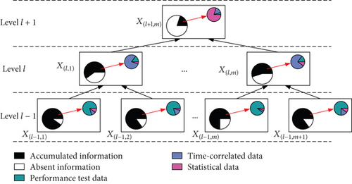
This article is organized as follows: In Section 2, the two critical issues of the MSDII system mentioned above are illustrated through a real harmonic gear drive (HGD) device and the rationale of the proposed information aggregation approach is introduced. And then, the Bayesian-based information aggregation process is discussed from both single-element and interelement aspects at full length in Section 3. Following that, in Section 4, a case study is demonstrated for validation, while the benefits and effectiveness of the proposal are also illustrated through a series of computations and comparisons. Finally, some concluding remarks are drawn in Section 5.

2. Problem Description of the MSDII System

The HGD device is the core part of the double-axis driving mechanism (DADM) which is used for erecting the antenna. In this paper, the HGD device is cited for instance to illustrate the two critical problems in the MSDII system. Its physical model is shown in Figure 2, and the system structure is represented by a hierarchical model in Figure 3. The whole device can be mainly divided into two subsystems, a spline system and harmonic wave generator. The spline system consists of a flexspline and a circular spline. The harmonic wave generator can be further decomposed into three components, that is, a wave generator producing basic torsion, a convex gear transmitting force and moment, and a direct current motor providing power.

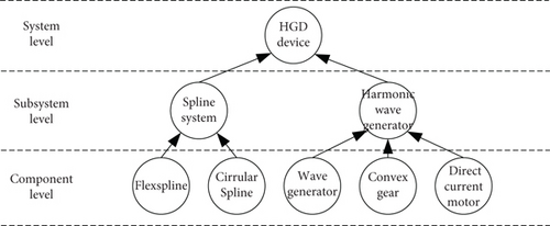
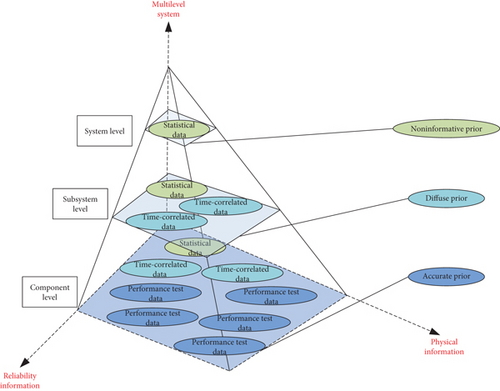
Figure 4 intuitively presents the scenario of multisource data and imbalanced information in the developing and manufacturing phases of the HGD. For basic components in the bottom level, we have abundant test data and sufficient prior knowledge. This prior information (e.g., judgment of experts, historical records of prototypes, and past experience of similar products) produces an informative and accurate prior probability distribution in the Bayesian inference. However, since the experiment for the system as a whole is both costly and time-consuming, test data is limited for higher-level elements. In addition, the prior knowledge is usually insufficient to construct an accurate and informative prior distribution; thus, the noninformative prior or diffuse prior is assigned on account of the scarce or even absent prior knowledge. Figure 4 gives a graphical description of the available information in the MSDII system, and Table 1 summarizes the characteristics of the three types of data (i.e., the statistical data, the time-correlated data, and the performance test data).

To balance the inadequacy of the available data, the Bayesian approach can be applied to explicitly incorporate prior knowledge into statistical modeling [4, 5]. The rationale of this framework is that based on the functional relationships of system elements, the lower-level reliability information can be explicitly aggregated to the system level and elicited as an attached probability index for the system reliability combination to compensate its information inadequacy. The detailed information aggregation procedure will be illustrated in the next section.

3. Bayesian-Based Multilevel and Multisource Data Fusion

This section presents the details of the proposed Bayesian-based information aggregation method, which is developed to resolve the reliability of a multilevel system with multisource data in an information imbalance scenario.

3.1. Single-Element Information Aggregation

3.1.1. BIC-Based Model Selection

In this section, a Bayesian information criterion- (BIC-) based model selection strategy is developed for single-element information aggregation. The HGD system shown in Figure 3 is considered here without loss of generality, in which the Bayesian network (BN) is constructed and shown in Figure 5.

• (i)

  For the statistical data (D^S) that only have the survival or failure records (e.g., pass/fail data and count data), the binomial distribution can be used to model the pass/fail data and the Poisson distribution can be adopted to model the count data set, as stated in [5, 23].

• (ii)

  For the time-correlated data (D^T) and performance test data (D^P), there is usually a number of candidate models (e.g., exponential, Weibull, and lognormal). In practical engineering, the model selection is a case-based procedure and the mathematical convenience should be taken into consideration. In this paper, the BIC is employed to help select an appropriate probability model among several candidates. The BIC (also named SBC and SBIC) is a criterion for model selection among finite sets of models, which is proposed by Schwarz [27] and further developed by Diciccio et al. [28].

The BIC has the following basic form:

$$ (1)

where x represents the observed data, n denotes the sample size, k refers to the number of free parameters, $$ is the likelihood function, and $$ denotes the estimation values that maximize the likelihood function. For a series of fixed test data, the smaller the BIC value is, the more acceptable the model is.

3.1.2. Likelihood Derivation for Heterogeneous Data Set

To build a comprehensive model for a multilevel system, heterogeneous data sets need to be incorporated. In this section, the likelihood contributions of the three types of data to the joint likelihood are derived.

(1) The Statistical Data Set. The statistical data set is defined as a data collection that only contains the dimensionless “number” information of the test unit or the element of interest. That is, the data set only records the number of units that survived or failed in an experiment or during a period of reality service time (e.g., the pass/fail data). Its mathematical form can be represented as a specification of D^S = D^S(N). From an information perspective, this type of data can only provide number information and is thought to be less informative compared with other types of data. Suppose that L units are subject to n_i independent sampling tests, where i = 1, …, L. The number of passing units in each test is x_i. Let X_i be the random variable following a binomial distribution. The probability that a unit passes the test is determined by its parameter $$. The model for X_i is described as

$$ (2)

The likelihood for a single observation (n_i, x_i) can be described as

$$ (3)

And the likelihood for the whole statistical data set is

$$ (4)

where all parameters in the statistical data set are involved in the parameter vector θ^S.

(2) The Time-Correlated Data Set. The time-correlated data set is defined as a type of data collection that contains both quantity and time information of a specific unit. For example, the failure time data gives exact records of failure time while the censored time data only provides partial information about failure time due to the limited test condition. Its mathematical form can be represented as the specification of a pair D^T = D^T(T, N), and it is thought that the time-correlated data is more informative than the simple statistical data. Eventually, the information obtained from a collection of time-correlated data is limited not only in the number of failures for a batch of tested units but also in the time point that a unit fails.

Various probability distributions can be used to model the time-correlated data set: exponential, Weibull and lognormal distribution have been employed in different research works [22, 23]. If the likelihood contribution of the exact failure time $$ is denoted as $$, the likelihood contribution of the left-censored time can be expressed as the cumulative distribution function (CDF) $$ while the likelihood contribution of the right-censored time $$ is derived similarly as $$. The likelihood function of the whole failure time data set could be obtained by multiplying the three individual contributions as

$$ (5)

where t^F, t^L, and t^R denote the exact time, left-censored time, and right-censored time of the failure, respectively, and n^F, n^L, and n^C denote the number of data points, respectively. All related parameters are involved in the parameter vector θ^T.

(3) The Performance Test Data Set. The performance test data set is defined as a type of data collection that records one kind of physical quantities which can reflect the performance of a product, for example, the starting acceleration of a motion mechanism and the output voltage of an electronic product. Its mathematical form can be represented as the specification of a triple D^P = D^P(G, N, T). Generally, the reliability refers to the capacity of a component or a system to perform its required functions under stated operating conditions during a specified period of time [29]. Failure occurs when the performance exceeds a predefined threshold as

$$ (6)

For a practical engineering problem, the reliability of one product is always related to multiple performance parameters and the reliability of this product is usually described as

$$ (7)

Equation (7) can be intuitively explained as follows: the reliability of one product is determined by the “worst” aspect in its performance.

From an information view, it is evident that the performance test data is much informative than the previous two types of data. This is because the performance test data provides not only the “outcome” information at the failure point but also the detailed “procedure” information. The most challenge in modeling this type of data is the difficulty in handling multisource data with different units (i.e., velocity and acceleration collected from a sensor and real-time monitoring voltage). To model all the performance test data in a coherent way, we transform all performance test data with nondimensional operation as

$$ (8)

where G_i(t = 0 | β) is the initial performance value which serves as the nondimensional operator. Based on (8), the performance function would begin with 100 percentile. Given the data measurement error ξ_i~Normal(0, σ²), the likelihood function for an individual data point at the time point t is

$$ (9)

where ϕ(⋅) is the probability density function (PDF) of the standard normal distribution. The G(t^P | β) denotes the value of a case-based performance function at the time point t^P. Taking the multiparameters at a series of time points t₁, t₂, …, t_n into consideration, the likelihood of the whole performance test data set is derived as

$$ (10)

where all parameters of the performance test data set are included in the parameter vector θ^P.

3.1.3. The Bayesian Model and Derivation of the Basic Probability Index

According to the Bayesian theorem, one-parameter posterior distribution is proportional to the multiplication of the likelihood function and the prior distribution. The joint likelihood function can be obtained by multiplying together the respective likelihood contributions of all available data sets. Let S^S, S^T, and S^P denote the sets of elements with statistical data, time-correlated data, and performance test data, respectively; then, the joint likelihood function is derived as

$$ (11)

where all parameters are involved in the parameter vector Θ. Given the prior distribution of the model parameter vector Θ, the Bayesian model is obtained as

$$ (12)

where π(Θ) is the joint prior distributions for the system model parameters and p(Θ | D^SD^TD^P) is the joint posterior distribution of the model parameter vector Θ.

There is usually no analytic solution to (12); however, the Markov chain Monte Carlo (MCMC) sampling techniques could be applied to get numerical solution (e.g., the Metropolis algorithms or the Gibbs samplers). The Metropolis random walk algorithm (MRWA) [30] is employed here to draw samples. Since the parameter vector Θ has been estimated, other reliability indexes could be evaluated by generating enough samples from the posteriors of parameters based on (13) and (14).

$$ (13)

$$ (14)

It should be noted that the information used to obtain the parameter posterior distribution from (12) and the reliability indexes from (13) and (14) is single-element based; namely, no additional information from interelements (e.g., other model outputs and system structural formation) is incorporated. Since the elements of a multilevel system are interconnected, it is desirable to aggregate all potential valuable information for reliability analysis and evaluation. On this occasion, we first estimate the parameters based on the two different data bases (i.e., the native information and induced information) and then integrate them into a comprehensive one. The probability indexes derived from (13) and (14) are defined as basic probability indexes, and the attached probability indexes on the basis of the interelement information will be discussed in the next section.

3.3. Summary of the MSDII System Information Aggregation Framework

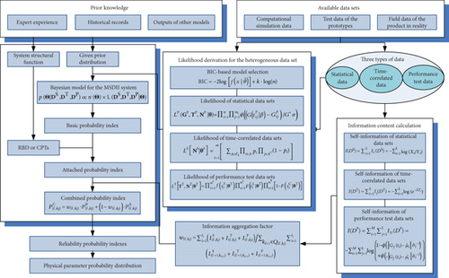
Several key steps of the proposed approach for the MSDII system are summarized as follows:

Step 1. Select the appropriate model based on the BIC calculation result.

Step 2. Derive the likelihood for elements with multisource data.

Step 3. Compute the basic probability indexes based on the native information.

Step 4. Calculate the attached probability indexes based on the induced information.

Step 5. Construct the combined probability indexes based on the information content of all available data sets.

Step 6. Estimate the probability indexes for reliability analysis or physical performance.

The flow diagram of the proposed approach is presented in Figure 6.

4. Numerical Case Study

4.1. Problem Description and Predefined Settings

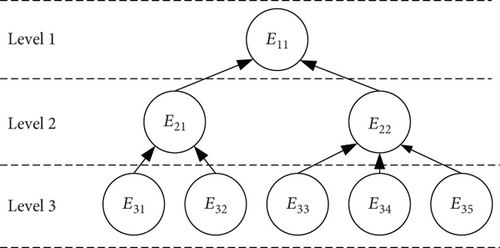
A numerical case study is conducted to illustrate the proposed information aggregation procedure and demonstrate its effectiveness in reliability estimation. The hierarchical HGD system is again investigated here. Figure 7 shows the HGD system structure considered in this section.

The traditional information aggregation methodology encounters an obstacle in reliability modeling and the analysis of the HGD system due to the existence of imbalanced information and multisource data. To illustrate, the available information of bottom-level components is well accumulated, which produces accurate prior knowledge. Nevertheless, the sub-system-level information is not always accessible due to the unaffordable cost of the entire system experiment; thus, the available information is strictly limited.

Case study settings are assumed on the basis of a real HGD system, but they are adjusted due to the confidentiality. Table 2 gives the predetermined probability indexes of bottom elements, and the detailed settings of all relevant CPTs are given in Table 3. Based on these, probability indexes of the remaining elements can be calculated, as shown in Table 4, where X = 1 denotes the normal state and X = 0 corresponds to the failure state. They will serve as the ground truth in the case study. To imitate an information imbalance scenario, the performance test data set with a sample size of 100, the time-correlated data set with a sample size of 50, and the statistical data set with a sample size of 10 (see details in Table 5) are randomly generated for components, subsystems, and the system-level elements, respectively, based on the ground truth. Additionally, accurate native priors are assigned to the components since the accumulated knowledge about them is abundant. For the sub-system-level elements, diffuse native priors are assigned considering the fact that only bounds of certain parameters can be determined. Because the prior knowledge is almost absent at the top system level, noninformative native priors are adopted.

Table 2. Predetermined bottom element probabilities.

Basic component elements	X = 1	X = 0
Pr(E31 = X)	0.97	0.03
Pr(E32 = X)	0.95	0.05
Pr(E33 = X)	0.80	0.20
Pr(E34 = X)	0.85	0.15
Pr(E35 = X)	0.90	0.10

Table 3. Predetermined CPTs.

	X = 1	X = 0
Interlevel CPT 1
Pr(E11 = X, E21 = 1, E22 = 1)	0.95	0.05
Pr(E11 = X, E21 = 1, E22 = 0)	0.70	0.30
Pr(E11 = X, E21 = 0, E22 = 1)	0.40	0.60
Pr(E11 = X, E21 = 0, E22 = 0)	0.10	0.90
Interlevel CPT 2
Pr(E21 = X, E31 = 1, E32 = 1)	1	0
…	…	…
Pr(E21 = X, E31 = 0, E32 = 0)	0	1
Interlevel CPT 3
Pr(E22 = X, E33 = 1, E34 = 1, E35 = 1)	1	0
…	…	…
Pr(E22 = X, E33 = 0, E34 = 0, E35 = 0)	0	1

Table 4. Calculated remaining element reliability.

Remaining system elements	X = 1	X = 0
Pr(E21 = X)	0.9215	0.0785
Pr(E22 = X)	0.9408	0.0592
Pr(E11 = X)	0.8918	0.1082

Table 5. Heterogeneous data sets used for the numerical case in Section 4 are displayed below. It is noted that all performance test data in various units have been nondimensionalized.

System level	Statistical data (time point)
E11	30/30 (0), 30/30 (1), 30/30 (2), 29/30 (3), 29/30 (4), 28/30 (5), 28/30 (6), 28/30 (7), 26/30 (8), 26/30 (9)
Subsystem level	Time-correlated data (“+” for censored time)
E21	387, 182, 244, 600, 627, 798, 660, 974, 1000+, 473, 954, 230, 464, 332, 418, 300, 584, 174, 50, 158, 345, 81, 1000+, 380, 131 ,1000+, 39, 274, 34, 1000+, 1000+
E22	130.3, 135.2, 152.4, 161.7, 74, 155, 141.2, 167.8, 137.2, 110.1, 200+, 200+, 200+, 200+, 190.5, 159.8, 200+, 192.4, 183.8, 200+
Component level	Performance test data (percentile)
Time point	0	1	2	3	4	5	6	7	8	9
E31 (transmission accuracy of the flexspline)	99.92	99.64	99.13	98.45	97.76	96.28	95.11	93.97	90.67	87.37
	99.97	99.36	99.24	98.87	97.13	95.96	94.88	93.46	90.13	86.48
E32 (transmission accuracy of the circular spline)	99.89		97.27		95.36		93.67		91.26
	99.25		97.84		95.07		93.83		91.58
	100.00		96.83		94.88		93.11		91.29
	99.73		97.14		95.89		94.03		91.94
E33 (output power of the wave generator)	99.47			90.26			75.47			59.15
	99.98			90.57			79.93			65.27
	99.65			89.24			80.35			64.76
	99.13			91.72			77.84			62.83
	99.32			90.24			76.19			61.66
E34 (transfer efficiency of the convex gear)	99.89			93.58			87.58			79.08
	99.76			93.97			87.87			80.01
	99.99			93.12			86.67			79.56
	99.97			94.16			88.13			81.29
	99.87			92.98			86.12			78.43
E35 (output power of the direct current motor)	99.45	99.12	98.85	98.34	97.82	97.39	96.84	96.34	95.68	94.97
	99.99	99.46	98.97	98.37	97.68	97.49	96.88	96.32	95.78	95.11

This case study is demonstrated to show how the proposed method improves the reliability evaluation result by using the imperfect information (i.e., inaccurate prior distribution and limited available data). The reliability framework for the case study is shown in Figure 8.

4.2. Bayesian-Based Information Aggregation Method and Reliability Estimation

4.2.1. Single-Element Information Aggregation

The multilevel information aggregation procedure starts with the model selection step. Since the available test data set for the system-level element is the nondimensional statistic data with a binary state, we use the binominal distribution to model the data set. For other elements, appropriate models are selected based on the computation of the BIC value among candidate distributions, and the calculated results are shown in Table 6.

Table 6. Calculation and selection of the likelihood function.

Element	Reliability data available	Data type	Calculated values based on BIC			Determined likelihood function
			Exponential	Weibull	Lognormal
E31	Performance test data	DP	136.0356	57.7402	54.7934	Lognormal distribution
E32	Performance test data	DP	135.7048	56.3441	55.5041	Lognormal distribution
E33	Performance test data	DP	22.5580	−6.9626	−10.5873	Lognormal distribution
E34	Performance test data	DP	21.0602	−16.0171	−16.7800	Lognormal distribution
E35	Performance test data	DP	19.6710	−16.7800	−18.6143	Lognormal distribution
E21	Time-correlated data	DT	223.2560	223.8714	228.2076	Exponential distribution
E22	Time-correlated data	DT	234.2629	233.5367	237.6452	Weibull distribution
E11	Statistic data	DS				Binominal distribution

Based on the likelihood constructed above, the basic probabilities (i.e., the reliability calculated using native information) are obtained from (13). These results are presented in Table 7. It is observed that the estimation results of component-level elements (E₃₁~E₃₅) are capable of high precision, whereas those of sub-system-level elements (E₂₁ and E₂₂) are of less accuracy. For system-level element (E₁₁), the result is significantly biased. Actually, the calculation of the basic probability using only native information has no essential difference compared with the traditional Bayesian-based approach. The traditional ones can get a satisfactory reliability analysis outcome in the ideal circumstance. However, the result would be biased if the prior is inaccurate or some data is misleading. Under the information imbalance scenario, it is desirable to use the components’ information to compensate the system information inadequacy for an improved reliability estimation. Thus, the interelement information aggregation is in demand.

Table 7. Reliability estimation after single-element information aggregation.

Element	Given prior distribution	Available test data (sample size)	Calculated reliability (native reliability)	Ground truth	Deviation
E31	Accurate, gamma (2.61, 120.57)	100	0.9999	0.97	3.08%
E32	Accurate, gamma (0.34, 47.51)	100	0.9773	0.95	2.87%
E33	Accurate, gamma (12.15, 56.3)	100	0.7530	0.8	5.88%
E34	Accurate, gamma (32.1, 100.57)	100	0.8626	0.85	1.48%
E35	Accurate, gamma (1.67, 87.45)	100	0.9403	0.9	4.48%
E21	Diffuse, normal (0, 1000)	50	0.7952	0.9215	13.71%
E22	Diffuse, beta (0.5, 0.5)	50	0.8393	0.9408	10.79%
E11	Noninformative, uniform (0, 1)	10	0.6628	0.8918	25.68%

4.2.2. Interelement Information Aggregation

Since the system structural function is presented by the CPT given in Table 3, the attached probabilities for higher-level elements of X₂₁, X₂₂, and X₁₂ can be calculated based on (15) as follows:

$$ (37)

Based on the derivations of self-information for heterogeneous data sets in (22), (23), (24), (25), (26), (27), (28), (29), and (30), the information content for elements with multisource data is obtained as

$$ (38)

Thus, the information aggregation factor is calculated as

$$ (39)

For the combined probability, we have

$$ (40)

It should be noted that P^C, P^B, and P^A in (22) are random variables with probability distribution. A direct way to calculate (40) is to apply the parameter combination by estimating an explicit form of the probability distribution first. However, it will bring more errors in the parameter estimation procedure. In this paper, we adopt a sample-based method by mixing samples generated from P^B and P^A to obtain enough random samples of P^C. In this way, no more deviation is introduced and an accurate combined probability is derived.

4.2.3. Result Analysis and Discussion

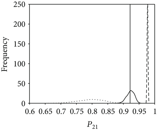
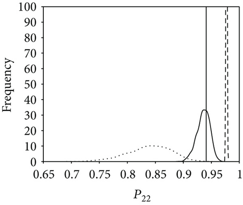
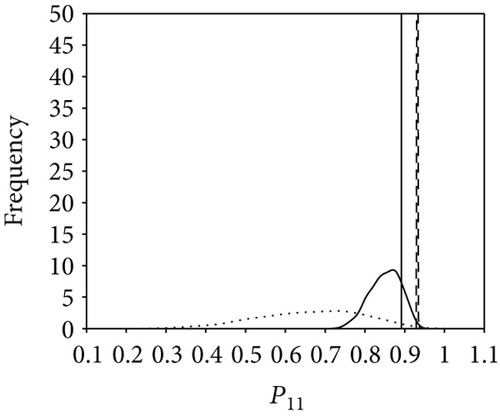
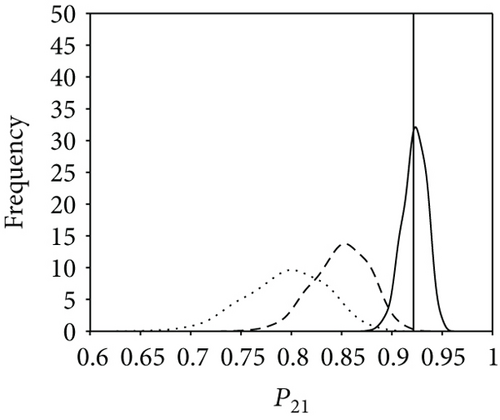
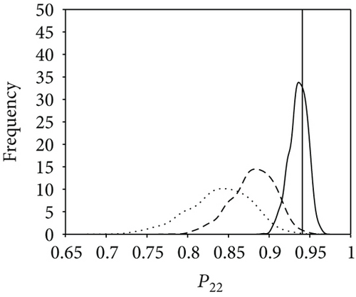
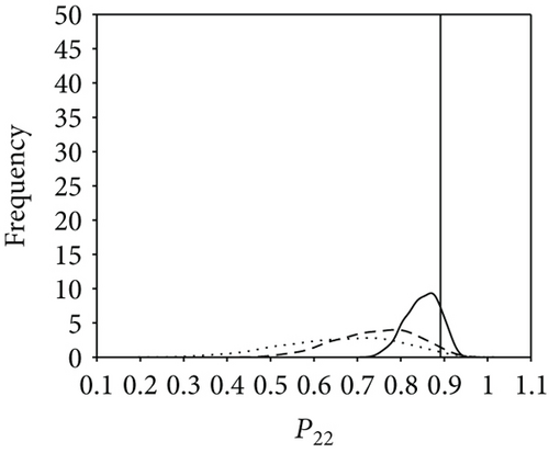
Figure 9 shows comparison results of the three posterior probability distributions (i.e., the basic probability, attached probability, and combined probability). For higher-level elements (E₂₁, E₂₂, and E₁₁), it appears that neither the basic probability nor the pure attached probability fits the ground truth well. By contrast, the combined probability shows a satisfactory result, indicating a successful proposal in reliability analysis of a multilevel system. Further, to validate the efficiency of our approach in uncertainty reduction, three subcases with different model specifications are presented; that is, only system-level information is utilized (less information aggregated with only statistical data), both system-level information and sub-system-level information are utilized (more information aggregated with statistical data and time-correlated data), and all available test data are employed (all information aggregated with three types of data). The comparison results of the three scenarios are shown in Figure 10, which suggests that as more information is aggregated, the estimation result is improved and the uncertainty is significantly reduced. Table 8 shows the 95% credible intervals and posterior mean and median of the reliabilities for E₂₁, E₂₂, and E₁₁. It can be seen that the 95% credible intervals fully cover the predetermined true value. The prior and posterior distributions of the failure rates λ₂₁ and λ₂₂ are calculated based on the (31) and (32) and listed in Table 9. The uncertainty reduction is calculated as (l_G − l_P)/l_G, where l_G and l_P are the 95% credible interval lengths of the probability distribution of parameters derived by the general Bayesian method and the proposed approach, respectively.

Table 8. Statistical results of posteriors for the subsystems and the whole system.

Element	Posterior mean	Posterior median	Ground truth	95% credible interval	Uncertainty reduction
P21	0.9225	0.9233	0.9215	[0.8977, 0.9429]	21.32%
P22	0.9358	0.9367	0.9408	[0.9111, 0.9553]	19.47%
P11	0.8510	0.8539	0.8918	[0.7686, 0.9162]	36.86%

Table 9. Statistical results of the failure rate for the subsystem elements.

Parameter	Prior mean	Posterior median	Ground truth	95% credible interval	Uncertainty reduction
λ21	1.069E − 3	8.051E − 4	8.1753E − 004	[5.749E − 4, 1.081E − 3]	18.82%
λ22	1.061E − 3	4.142E − 4	3.8140E − 004	[2.8E − 4, 5.79E − 4]	31.37%

Note that we have made some assumptions in this case study. They are acceptable in this numerical case for validation purpose, but it may require some additional considerations in practical engineering. For example, we do not consider the model uncertainty; that is to say, we assume that the established model (system configuration) is in complete accordance with the ground truth; for a practical engineering problem, the simulation model should be validated by the physical model before the approach is implemented. In addition, we assume that the used data is accurately obtained; thus, the measurement error is omitted; likewise, the collected data should be carefully calibrated before it is aggregated in the Bayesian model since it can significantly affect the estimation result. For relevant research works, please refer to [14–16].

5. Conclusion

This article proposes a multilevel information aggregation approach to evaluate the reliability of an MSDII system accurately, addressing two crucial issues in engineering reliability evaluation, that is, the imbalanced information and multisource data fusion. Based on system structural function, the reliability information of component-level elements has been aggregated to compensate the information inadequacy of the system level, yielding a better effect on the reliability analysis of the whole system. A real HGD system is demonstrated to confirm the validity and effectiveness of the proposal. The improved system reliability modeling will benefit system prognosis, warranty policy making, and the maintenance service planning, providing a more reliable assessment of the system’s health status with more accurate prediction of the remaining useful life. Furthermore, some better predictive maintenance policies can be established with less uncertainty.

It should be noted that our approach is developed for a coherent system; namely, this approach is feasible for series systems, parallel systems, k-out-n systems, and so on, but some complex systems do not fall within the scope of application. Since the structure function of some complex systems is not in analytical form or cannot be explicitly expressed, (15) and (16) are not applicable. It is also noted that many inherent uncertain factors in practical engineering such as model uncertainty, measurement error, and the cascading failure dependency have not been taken into consideration. A full Bayesian approach dealing with both aleatory uncertainties and epistemic uncertainties with cascading failure dependency would be under the consideration of the future work. It will be interesting to compare the frequency-based and full Bayesian approaches in the future from different aspects such as computational complexity, modeling accuracy and precision, and data availability and quality.

Conflicts of Interest

The authors declare that they have no conflicts of interest.