This paper presents space-time kriging within a multi-Gaussian framework for time-series mapping of particulate matter less than 10 μm in aerodynamic diameter (PM₁₀) concentration. To account for the spatiotemporal autocorrelation structures of monitoring data and to model the uncertainties attached to the prediction, conventional multi-Gaussian kriging is extended to the space-time domain. Multi-Gaussian space-time kriging presented in this paper is based on decomposition of the PM₁₀ concentrations into deterministic trend and stochastic residual components. The deterministic trend component is modelled and regionalized using the temporal elementary functions. For the residual component which is the main target for space-time kriging, spatiotemporal autocorrelation information is modeled and used for space-time mapping of the residual. The conditional cumulative distribution functions (ccdfs) are constructed by using the trend and residual components and space-time kriging variance. Then, the PM₁₀ concentration estimate and conditional variance are empirically obtained from the ccdfs at all locations in the study area. A case study using the monthly PM₁₀ concentrations from 2007 to 2011 in the Seoul metropolitan area, Korea, illustrates the applicability of the presented method. The presented method generated time-series PM₁₀ concentration mapping results as well as supporting information for interpretations, and led to better prediction performance, compared to conventional spatial kriging.

1. Introduction

Outdoor air pollution has been known as one of the risk factors that affect human health directly and/or indirectly [1–4]. In Korea, it is reported that long-term exposure to ambient air pollution has a reasonable association with tuberculosis, cardiovascular diseases, and preterm delivery [5–7]. Thus, periodic monitoring and management of air pollution are required for exposure assessment for effective health management.

In Korea, several air pollutants including particulate matter less than 10 μm in aerodynamic diameter (PM₁₀), sulfur dioxide (SO₂), carbon monoxide (CO), nitrogen dioxide (NO₂), ozone (O₃), and particulate matter less than 2.5 μm in aerodynamic diameter (PM_2.5) have been periodically collected at several monitoring stations. Based on this real-time monitoring of air pollution, air quality levels are provided to the public domain [8]. Due to the few stations, however, it is very difficult to analyze the spatial characteristics and spatiotemporal dynamics of air pollutants over a wide study area during the predefined time interval [9]. To overcome these difficulties, spatial interpolation or prediction is routinely applied to the sparse air pollutants observations to obtain exhaustive concentration values over the study area.

Among various spatial interpolation methods, geostatistical kriging has been widely applied to spatial interpolation tasks, due to its ability to account for spatial autocorrelation structures inherent to sample data and to integrate auxiliary data [10, 11]. When kriging is applied for spatial interpolation, spatial autocorrelation structures are quantified by variogram which denotes the spatial variability between samples as a function of distance [10]. If only sparsely sampled data are available, distinct spatial autocorrelation structures may not be captured from the sample data. As a result, spatial interpolation results would not show better prediction performance, compared to other deterministic interpolation methods such as inverse distance weighting. If data are collected at a limited number of locations but continuously in a time domain such as air pollutants, temperature, and precipitation, temporal autocorrelation information may complement the lack of spatial autocorrelation information and improve the prediction performance for spatial interpolation tasks. Regarding the processing of this kind of space-poor but time-rich data, conventional geostatistical kriging, which was developed for considering spatial autocorrelation information only, can be extended to space-time kriging [12]. Space-time kriging or simulation has been applied to time-series mapping of various environmental variables such as air pollutants, temperature, and precipitation [13–16]. Despite its great potential for time-series mapping, however, uncertainties attached to the interpolation have not been fully accounted for. Most approaches have focused on the generation and interpretation of spatiotemporal mapping results. To the author’s knowledge, very few studies have been conducted using stochastic simulation [14] and local uncertainty assessment based on space-time kriging that does not require heavy computational cost is not fully considered. Recently, Park [17] presented a multi-Gaussian framework for time-series mapping of environmental variables. As the case study in [17] was carried out in the very small area, however, its applicability should be thoroughly investigated.

The main objective of this paper is to present space-time kriging capable of providing uncertainty assessment information and time-series mapping of PM₁₀ concentrations. Within a spatial time-series framework [14, 17], conventional spatial multi-Gaussian kriging is extended to a space-time domain and its potential is illustrated via a case study of monthly PM₁₀ concentration mapping in the Seoul metropolitan area, Korea.

2. Study Area and Data

A case study was conducted in the Seoul metropolitan area of Korea which includes 66 provincial districts in Seoul city, Incheon city, and Gyeonggi province (Figure 1). The metropolitan area covers approximately 11.78% of the entire land area of Korea and accounts for 49.07% of the entire population of Korea, as of 2014 and 2010, respectively [7, 18]. The study area comprised various types of land-covers, including the large urban areas of Seoul city and Incheon city located in the central and western parts of the study area, and the forests and agricultural lands (78.46% of the whole study area) located in the northern and eastern parts of the study area.

Details are in the caption following the image — **Figure 1**
Open in figure viewer PowerPoint

Locations of the study area and PM₁₀ monitoring stations (black dots) with administrative boundaries.

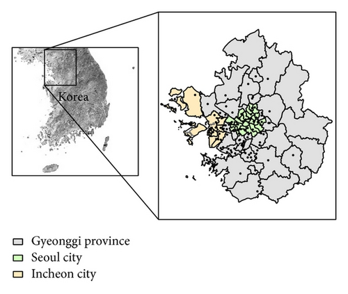
A monthly PM₁₀ concentration dataset collected at 94 monitoring stations in the study area from January 2007 to December 2011 (60 months) was downloaded from the AirKorea website [8] and used for the case study. As shown in Figure 1, each district in the Seoul metropolitan city includes one station, but there are very few monitoring stations in other districts in Gyeonggi province, which comprised nearly half (47.74%) of the study area. This location information on the monitoring stations implies that relatively large uncertainties may be attached to the sparsely sampled locations. Within the administrative boundaries, 500 m interval grid points were generated and PM₁₀ concentrations were mapped at these points. It should be noted that the main purpose of this case study is to exemplify the analytical procedures and potential of the geostatistical approach presented in this paper, not to reveal detailed local characteristics of PM₁₀ concentrations in the study area.

3. Method

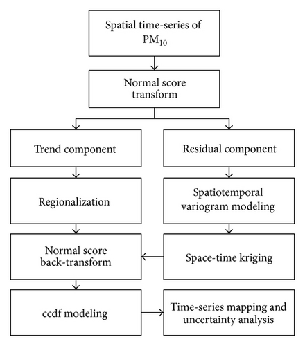
Figure 2 illustrates the entire procedure for the multi-Gaussian spatial time-series approach presented in this paper.

3.1. Multi-Gaussian Spatial Time-Series Approach

The time-series PM₁₀ concentration at each observation station was regarded as spatial time-series data and these spatial time-series datasets were modelled as spatially correlated time-series random function models [14, 17]. Suppose that {Z(u, t), t ∈ T, u ∈ S} denotes the spatially indexed time-series PM₁₀ concentrations within the discrete time domain T and the continuous space domain S. In geostatistics, the uncertainty at any unmonitored location is usually modeled through the conditional cumulative distribution function (ccdf) which states the probability that the unknown attribute value does not exceed a certain threshold value z [10]. If this ccdf is extended to a space-time domain, the uncertainty at a certain location u and time t is modeled via the following ccdf of Z(u, t):

()

where “∣(info)” denotes conditioning to the local neighboring data both spatially and temporally.

In this study, multi-Gaussian space-time kriging was adopted for ccdf modeling as a parametric approach. Under the assumption that the ccdf at any location u follows a Gaussian or normal distribution, the multi-Gaussian approach aims to predict the mean and variance, which are the two parameters that define the Gaussian ccdf [10]. To satisfy the assumption of a Gaussian ccdf, all monitoring data are transformed into a Gaussian space by normal score transform [11]. Then, the transformed spatial time-series dataset (Y) will follow a standard Gaussian distribution with a mean of 0 and a standard deviation of 1, and its ccdf is expressed as

()

where G[ ] is a standard Gaussian cumulative distribution function. E{Y(u, t)∣(info)} and Var⁡{Y(u, t)∣(info)} are mean and variance values obtained by using the given neighboring data, respectively. These two values, which are required to define the Gaussian distribution, correspond to the simple kriging estimate and simple kriging variance, respectively.

To fully characterize the ccdf in (2), PM₁₀ concentrations were modelled by decomposing the data into a deterministic trend component and a stochastic residual component [14, 17, 19]. The trend component is related to overall PM₁₀ concentration patterns such as seasonal or regional variations. Meanwhile, the residual component, which is regarded as a second-order stationary random variable, includes local variations of PM₁₀ concentration at a certain time and location and is the main target of geostatistical analysis. Since the multi-Gaussian approach was adopted in this study, this decomposition was applied to the normal score transformed dataset like

()

where m_G(u, t) and R_G(u, t) denote the trend and residual components in a Gaussian space, respectively.

3.2. Trend Component Modeling

The trend component in (3) was modelled by weighted linear combination of elementary temporal profile functions presented in [14]. Suppose that Y(u_α, t_β) is a normal score transformed PM₁₀ concentration at a certain monitoring station during the time period of 60 months (α = 1, …, 94, β = 1, …, 60). The trend component at the αth monitoring station (m_G(u_α, t_β)) is expressed as a weighted sum of elementary temporal profile functions. Many elementary temporal profile functions can be applied for trend modeling. For example, periodicity and linear trend can be accounted for by combining linear and trigonometric functions. In this study, a spatially averaged time-series set computed from 94 monitoring stations [14] was used as the elementary temporal profile function for its simplicity:

()

where a₀ and a₁ correspond to the intercept and slope, respectively, in linear regression and are related to the similarity between a normal score transformed time-series at a certain monitoring station and the spatially averaged time-series set.

The above two regression coefficients are only available at monitoring stations after linear regression. Thus, they should be interpolated at all grid points in the study area for all time intervals in order to obtain the trend component distributions. If reasonable correlations are observed between two coefficients, simple cokriging, which can account for both the autocorrelation structures of the two coefficients and the cross-correlation structure between them, can be applied for spatial interpolation. Otherwise, univariate kriging or another deterministic interpolation method is independently applied to each coefficient. After regionalization or interpolation of the two coefficients, a trend component over the study area at each month was obtained by combining the interpolated coefficients with the spatially averaged time-series set.

3.3. Residual Component Modeling

The residual components, which are regarded as the second-order stationary random variable and subject to the main geostatistical analysis, were modelled via space-time kriging.

Spatiotemporal correlation structures required for the application of space-time kriging were first quantified via variogram modeling. The experimental spatiotemporal variogram is defined as

()

where h_s and h_t denote spatial lag distance and temporal interval, respectively, and N(h_s, h_t) is the number of data pairs within the class of spatiotemporal lags.

Among various spatiotemporal variogram models, a product-sum variogram model in [20] was applied to model the experimental spatiotemporal variogram. The product-sum variogram model is expressed as the combination of marginal spatial and temporal variograms (i.e., purely spatial variogram and purely temporal variogram) as [20]

()

where γ_s is the marginal spatial variogram and γ_t the marginal temporal variogram. C_s(0) and C_t(0) are the sill values of γ_s and γ_t, respectively.

Some parameters in (6) are also defined as [21]

()

where C_st(0,0) is a sill value of the spatiotemporal variogram model.

After completion of the spatiotemporal variogram modeling, the residual components at all grid points in the study area for all time intervals were obtained by a linear combination of neighboring sample residual values within the predefined spatiotemporal search window via simple space-time kriging. The simple space-time kriging estimate

and variance

were computed as

()

where λ_α(u, t) is a simple kriging weighting value assigned to the neighboring sample residuals and C_st(u_α − u, t_α − t) is a spatiotemporal covariance value between the estimation grid and neighboring sample locations. Since the residuals have a zero mean value, a constant mean value required for simple kriging is set to 0 and does not appear in (8).

3.4. ccdf Modeling

The space-time kriging estimate and variance for the residuals were used for fully characterizing the ccdf in a Gaussian space in (2). More specifically, the residual estimate at any grid point was added to the trend component at the corresponding grid point and then used as a mean value of the ccdf. Since the trend component was assumed to be deterministic, the space-time kriging variance was directly used as the variance value of the ccdf.

The ccdfs at all grid points in the study area were already fully known after applying the normal score back-transform. Then, certain statistics could be used as PM₁₀ concentration estimates and uncertainty measures. The PM₁₀ concentration value (z^∗(u, t)) was empirically estimated from the expected value of the corresponding normal score back-transformed quantiles in the original space after discretizing the ccdf with many p quantiles (y_p(u, t)) in the Gaussian space, as presented in [22, 23]

()

where F⁻¹[G(y_p(u, t))] denotes the normal score back-transformed values of the p quantiles in the Gaussian space.

Like the computation of the expected value of the ccdf, conditional variance (σ^2∗(u, t)) was also computed using (10) [23] and used as a measure of uncertainty:

()

Unlike kriging variance that provides only the proximity from the sample data, conditional variance can provide information on the spread of the conditional probability distribution function or the steepness of the ccdf and thus can be used as a quantitative measure of the uncertainty. The larger the conditional variance, the greater the uncertainty attached to the prediction.

In addition to the computation of PM₁₀ concentration estimates and uncertainty measures from the ccdf, a probability of exceeding a certain critical concentration level can be easily computed. Based on this probability and the PM₁₀ concentration estimates, misclassification risks, which are associated with the classification of the study areas into hazardous and safe classes, can be computed and then used for decision supporting information.

Two misclassification risks α and β were considered in this study. Risk α, which is the probability of wrongly classifying any location u as hazardous (i.e., false positive), is defined as [10]

()

where z_k is a critical PM₁₀ concentration level.

Risk β, which is a probability of wrongly classifying any location u as safe (i.e., false negative), is given as [10]

()

3.5. Validation

The prediction performance of multi-Gaussian space-time kriging was quantitatively evaluated by leave-one-out cross validation since kriging is an exact interpolator. After one monitoring station was temporarily eliminated, kriging using the remaining stations was conducted to predict the PM₁₀ concentration at the eliminated monitoring station. This procedure was repeated for all monitoring stations. Then the prediction performance was quantified using the linear correlation coefficient between the true PM₁₀ concentration and the mean absolute error (MAE).

4. Results and Discussion

4.1. Trend Component Modeling Result

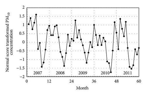
After preparing time-series PM₁₀ concentration datasets, normal score transform was first applied using GSLIB [11]. Figure 3 shows a spatially averaged time-series that was computed from normal score transformed PM₁₀ concentrations and used as the elementary temporal profile function. During the 5-year period from 2007 to 2011, a decreasing pattern was observed from April to August, but the increase in PM₁₀ concentration commenced in fall and continued to winter. However, the winter PM₁₀ concentration exhibited a different pattern each year. This overall pattern may be related to yellow dust in spring and meteorological factors such as wind, relative humidity, and precipitation. In winter and spring, the relatively stable atmospheric condition with high relative humidity and yellow dust contributes to the increase in PM₁₀ concentration, respectively; meanwhile, the low PM₁₀ concentration in summer is due to the washout effect by precipitation, as reported in previous studies [24, 25].

Regression between the spatially averaged time-series set and the time-series set at each monitoring station was conducted and two regression coefficients are presented in Figure 4. If the intercept and slope values approach zero and one, respectively, the time-series at the monitoring station is very similar to the spatially averaged time-series set. The different similarities at the monitoring stations led to differences of trend components, and hence the residual components, which are the main targets of space-time kriging, also varied across the study area.

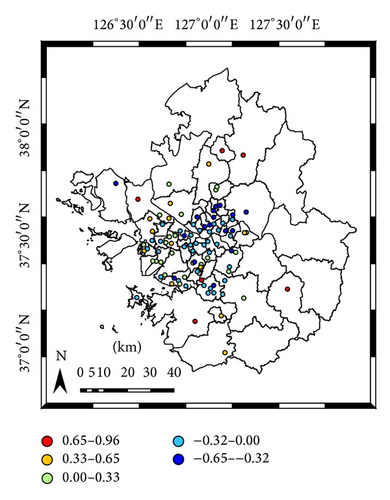
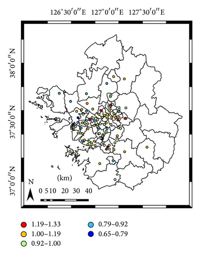
The next step for the regionalization or estimation of trend components at unmonitored locations was to interpolate the intercept and slope values in Figure 4. The linear correlation coefficient between the two coefficients at 94 monitoring stations was very low (−0.08), so an independent univariate ordinary kriging was applied to the two coefficients. By combining the interpolated regression coefficients with the spatially averaged time-series set in Figure 3, the trend components during the considered time period were retrieved and used for ccdf modeling.

4.2. Residual Component Modeling Result

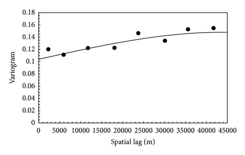
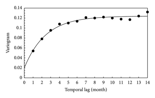
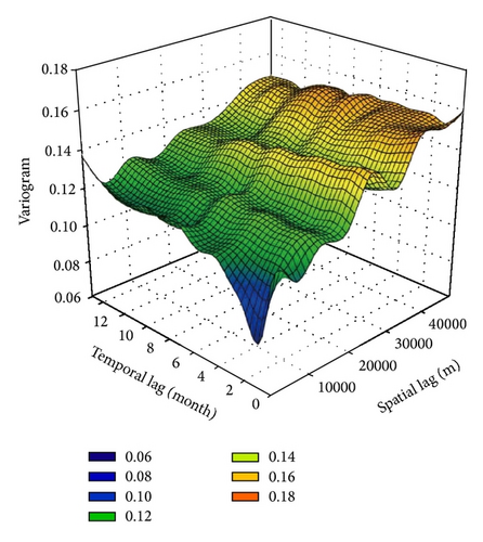
After computing trend components at each monitoring station, the residual components that could not be explained by the trend components were computed at each monitoring station. The modified Fortran routines of De Cesare et al. [21] were used to compute the experimental spatiotemporal variogram. The marginal spatial and temporal experimental variograms of the residuals with the fitted models are given in Figures 5(a) and 5(b), respectively. The marginal spatial variogram (Figure 5(a)) showed large relative nugget effects, but a reasonable temporal autocorrelation structure with an effective range of about 7 months was observed in the marginal temporal variogram (Figure 5(b)). This result implies that to account for temporal autocorrelation information during the interpolation could improve prediction performance, compared to the interpolation case with only spatial autocorrelation information. Figure 5(c) presents the experimental spatiotemporal variogram surface of the residuals. From this figure, the spatiotemporal variogram model, which satisfies the constraints in (8), was finally estimated and then used as an input variogram model for space-time kriging. Space-time kriging was applied to obtain the residuals at all grid points in the study area by using the spatiotemporal variogram model of the residuals. The Edinburgh space-time geostatistics Fortran program [26] was used to implement space-time kriging of the residuals.

4.3. PM₁₀ Concentration Mapping and Uncertainty Analysis Results

The simple space-time kriging estimate of the residuals was added to the interpolated trend components and then used as a mean value for the Gaussian ccdf at all locations. The simple space-time kriging variance was also used as the variance of the Gaussian ccdf, as in (2). After constructing ccdfs at all locations, the PM₁₀ concentration estimate and conditional variance were computed using (9) and (10), respectively. All postprocessing was implemented by Fortran programming and ArcGIS was used for visualization.

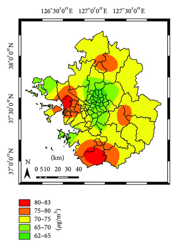
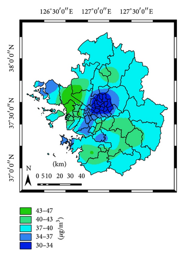
Only the PM₁₀ concentration mapping results for two months in 2011 are given in Figure 6, due to space limitation. The PM₁₀ concentration in April was much higher than that in August due to less precipitation and yellow dust transported to Korea by prevailing westerly winds in April. In April, relatively high PM₁₀ concentrations were observed in northern Incheon, Dongducheon, Pyeongtaek, and Gwangju due to the large concentrations either at the monitoring stations in those cities or at the nearby monitoring stations. The PM₁₀ concentration in August was relatively high in the northern Incheon, Gimpo, Dongducheon, Hwaseong, Seongnam, Gwangju, and northern Icheon. In both months, the northern Incheon, Dongducheon, and Gwangju showed relatively high concentrations, but low concentrations were observed in Seoul city.

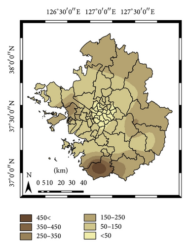
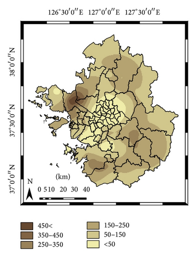
The spatial distribution of conditional variance that measures the uncertainty for prediction is given in Figure 7. A large conditional variance was observed in some concentration areas (e.g., northern Incheon and Pyeongtaek in April and Gimpo in August, resp.) where the PM₁₀ concentration values at monitoring stations fluctuated greatly both temporally and spatially. Some areas with very few or even no monitoring showed relatively large conditional variance which is similar to conventional kriging variance. This uncertainty statistic revealed that the conditional variance, which provides information on both the sample variations and the sample configuration, can be used as supporting information to interpret the PM₁₀ concentration mapping result.

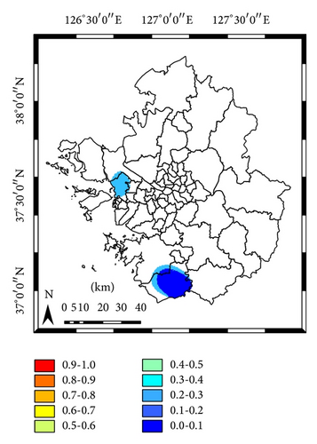
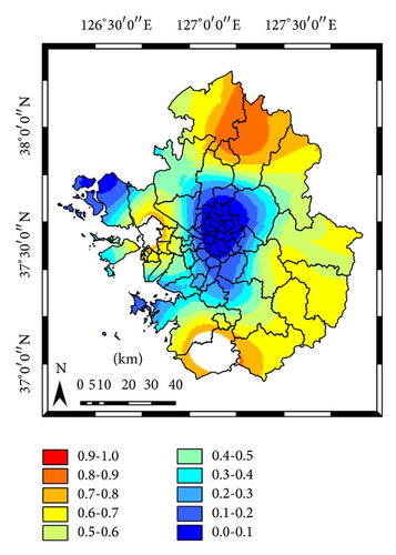
To generate misclassification risk maps, the probability of exceeding a certain threshold value was first mapped. The atmospheric environmental standard in Korea is defined only for an annual average (25 μm/m³) or a 24-hour average (100 μm/m³) [8]. Thus, it is not feasible to directly use the atmospheric environmental stand value as the threshold, since the monthly PM₁₀ concentration was considered in this study. Since the ccdfs were established at all locations in the study area, a variety of probability maps could easily be generated by applying different threshold values. For an illustration purpose, the PM₁₀ concentration of 80 μm/m³ was used as the threshold. By combining the classification result with the exceeding probability using a PM₁₀ concentration of 80 μm/m³ as the critical threshold, the risk α and risk β maps were generated, as shown in Figure 8. By definition, risk α is only mapped where the PM₁₀ concentration exceeds the predefined threshold. On the contrary, risk β is defined where risk α is not mapped. In the risk α map in Figure 8(a), the false positive probability is relatively low (i.e., less than 0.3), but not negligible. The risk β map in Figure 8(b) shows very large variations of the false negative probability, which is greater than 0.7 in the northern part of the study area including Pocheon and Yeoncheon. A large misclassification risk β was also found around the areas that are classified as hazardous (i.e., exceeding the PM₁₀ concentration of 80 μm/m³). Although choosing proper probability thresholds is difficult or subjective, these misclassification risk maps, which cannot be provided by deterministic interpolation methods or kriging algorithms without ccdf modeling, can be useful information for further decision-making or interpretations. For example, the areas showing high misclassification risk values can be considered as candidates for further monitoring or in-depth investigations.

4.4. Validation Results

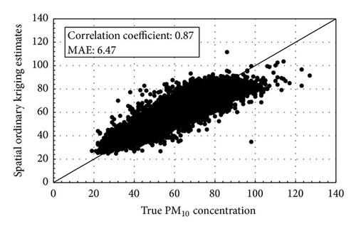
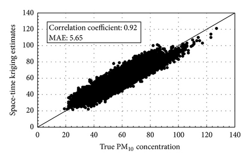
To quantitatively evaluate the prediction performance of space-time kriging, leave-one-out cross validation was carried out and error statistics such as the linear correlation coefficient with the true values and MAE were computed. Spatial ordinary kriging, which considers only spatial autocorrelation information, was also applied for comparison purpose.

Figure 9 presents the scatter-plots with error statistics computed from leave-one-out cross validation. Although the underestimation of high values and overestimation of low values were observed in both results, this mismatch arising from the smoothing effects of kriging was relatively weakened in the validation result of space-time kriging. The linear correlation coefficients for space-time kriging and spatial ordinary kriging were 0.92 and 0.87, respectively. Space-time kriging also showed an improvement of 13.23% in MAE, compared to that of spatial ordinary kriging. Similar to the previous case study result in Park [17], these quantitative evaluation results confirmed that the incorporation of temporal autocorrelation information via space-time kriging improved the prediction performance and generated reliable mapping results for space-poor and time-rich data such as PM₁₀ concentrations.

5. Conclusions

A geostatistical approach based on spatiotemporal multi-Gaussian kriging was presented for time-series mapping of PM₁₀ concentrations. Unlike conventional space-time kriging and spatial kriging, which provide the estimate and kriging variance only, the presented approach generated rich interpretable by-products as well as the PM₁₀ estimates. From a case study in the Seoul metropolitan area of Korea, multi-Gaussian space-time kriging accounted for temporal autocorrelation information as well as spatial autocorrelation information and generated reliable mapping results that outperformed those of conventional spatial kriging. In addition, the presented approach produced uncertainty measures and misclassification risks from the ccdf modeling that are useful for interpretation or decision-making.

To strengthen the major findings of this study, several outstanding issues should be addressed in future work. First, several auxiliary variables such as the proximity to major roads and weather data will be integrated within the framework of the present study in order to generate much more reliable PM₁₀ concentration mapping results. In relation to uncertainty modeling, the multi-Gaussian approach adopted herein may not be appropriate for datasets with a strong positively skewed distribution which may be often observed in air pollutant concentrations. Thus, the extension of the conventional spatial indicator approach [10, 11] to the space-time domain and the comparison with the multi-Gaussian approach presented herein will also be included in future work.

Conflict of Interests

The author declares that there is no conflict of interests regarding the publication of this paper.

Acknowledgments

This research was supported by Basic Science Research Program through the National Research Foundation of Korea (NRF) funded by the Ministry of Science, ICT & Future Planning (NRF-2015R1A1A1A05000966). This work was also supported by Inha University Research Grant. The author thanks Dr. L. Spadavecchia for providing the Edinburgh space-time geostatistics program.

References

1 Kaiser J., How dirty air hurts the heart, Science. (2005) 307, no. 5717, 1858–1859, 2-s2.0-15744370671.
10.1126/science.307.5717.1858a
PubMed Web of Science® Google Scholar
2 Medina-Ramón M., Zanobetti A., and Schwartz J., The effect of ozone and PM₁₀ on hospital admissions for pneumonia and chronic obstructive pulmonary disease: a national multicity study, The American Journal of Epidemiology. (2006) 163, no. 6, 579–588, https://doi.org/10.1093/aje/kwj078, 2-s2.0-33644893664.
10.1093/aje/kwj078
PubMed Web of Science® Google Scholar
3 Ghosh J. K. C., Wilhelm M., Su J., Goldberg D., Cockburn M., Jerrett M., and Ritz B., Assessing the influence of traffic-related air pollution on risk of term low birth weight on the basis of land-use-based regression models and measures of air toxics, American Journal of Epidemiology. (2012) 175, no. 12, 1262–1274, https://doi.org/10.1093/aje/kwr469, 2-s2.0-84862506259.
10.1093/aje/kwr469
PubMed Web of Science® Google Scholar
4 Carbajal N., Pineda-Martinez L. F., and Vicente F. B., Air quality deterioration of urban areas caused by wildfires in a natural rservoir forest of Mexico, Advances in Meteorology. (2015) 2015, 13, 912946, https://doi.org/10.1155/2015/912946.
10.1155/2015/912946
Web of Science® Google Scholar
5 Hwang S.-S., Kang S., Lee J.-Y., Lee J. S., Kim H. J., Han S. K., and Yim J.-J., Impact of outdoor air pollution on the incidence of tuberculosis in the Seoul metropolitan area, South Korea, Korean Journal of Internal Medicine. (2014) 29, no. 2, 183–190, https://doi.org/10.3904/kjim.2014.29.2.183, 2-s2.0-84897831743.
10.3904/kjim.2014.29.2.183
CAS Web of Science® Google Scholar
6 Leem J.-H., Kaplan B. M., Shim Y. K., Pohl H. R., Gotway C. A., Bullard S. M., Rogers J. F., Smith M. M., and Tylenda C. A., Exposures to air pollutants during pregnancy and preterm delivery, Environmental Health Perspectives. (2006) 114, no. 6, 905–910, https://doi.org/10.1289/ehp.8733, 2-s2.0-33745024505.
10.1289/ehp.8733
CAS PubMed Web of Science® Google Scholar
7 Lim Y.-R., Bae H.-J., Lim Y.-H., Yu S., Kim G.-B., and Cho Y.-S., Spatial analysis of PM₁₀ and cardiovascular mortality in the Seoul metropolitan area, Environmental Health and Toxicology. (2014) 29, e2014005, https://doi.org/10.5620/eht.2014.29.e2014005.
10.5620/eht.2014.29.e2014005
PubMed Google Scholar
8 AirKorea, http://www.airkorea.or.kr/.
Google Scholar
9 Zou B., Luo Y., Wan N., Zheng Z., Sternberg T., and Liao Y., Performance comparison of LUR and OK in PM_2.5 concentration mapping: a multidimensional perspective, Scientific Reports. (2015) 5, article 8698, https://doi.org/10.1038/srep08698.
10.1038/srep08698
Web of Science® Google Scholar
10 Goovaerts P., Geostatistics for Natural Resources Evalution, 1997, Oxford University Press, New York, NY, USA.
10.1093/oso/9780195115383.001.0001
Google Scholar
11 Deutsch C. V. and Journel A. G., GSLIB: Geostatistical Software Library and User′s Gudie, 1998, Oxford University Press, New York, NY, USA.
Google Scholar
12 Kyriakidis P. C. and Journel A. G., Geostatistical space-time models: a review, Mathematical Geology. (1999) 31, no. 6, 651–684, https://doi.org/10.1023/A:1007528426688, MR1694654, ZBL0970.86013, 2-s2.0-0032752472.
10.1023/A:1007528426688
Web of Science® Google Scholar
13 De Iaco S., Myers D. E., and Posa D., Space-time variograms and a functional form for total air pollution measurements, Computational Statistics and Data Analysis. (2002) 41, no. 2, 311–328, https://doi.org/10.1016/s0167-9473(02)00081-6, MR1945873, 2-s2.0-0037192052.
10.1016/S0167-9473(02)00081-6
Web of Science® Google Scholar
14 Kyriakidis P. C., Miller N. L., and Kim J., A spatial time series framework for simulating daily precipitation at regional scales, Journal of Hydrology. (2004) 297, no. 1–4, 236–255, https://doi.org/10.1016/j.jhydrol.2004.04.022, 2-s2.0-3242763977.
10.1016/j.jhydrol.2004.04.022
Web of Science® Google Scholar
15 Fernández-Cortés A., Calaforra J. M., Jiménez-Espinosa R., and Sánchez-Martos F., Geostatistical spatiotemporal analysis of air temperature as an aid to delineating thermal stability zones in a potential show cave: implications for environmental management, Journal of Environmental Management. (2006) 81, no. 4, 371–383, https://doi.org/10.1016/j.jenvman.2005.11.011, 2-s2.0-33750022610.
10.1016/j.jenvman.2005.11.011
CAS PubMed Web of Science® Google Scholar
16 Spadavecchia L. and Williams M., Can spatio-temporal geostatistical methods improve high resolution regionalisation of meteorological variables?, Agricultural and Forest Meteorology. (2009) 149, no. 6-7, 1105–1117, https://doi.org/10.1016/j.agrformet.2009.01.008, 2-s2.0-62849105579.
10.1016/j.agrformet.2009.01.008
Web of Science® Google Scholar
17 Park N.-W., Time-series mapping and uncertainty modeling of environmental variables: a case study of PM₁₀ concentration mapping, Journal of the Korean Earth science Society. (2011) 32, no. 3, 249–264, https://doi.org/10.5467/jkess.2011.32.3.249.
10.5467/JKESS.2011.32.3.249
Google Scholar
18 Korean Statistical Information Service (KOSIS), http://kosis.kr/.
Google Scholar
19 Diggle P. J. and Ribeiro P. J., Model-Based Geostatistics, 1998, Springer, New York, NY, USA.
Google Scholar
20 De Cesare L., Myers D., and Posa D., Product-sum covariance for space-time modeling: an environmental application, Environmetrics. (2001) 12, no. 1, 11–23, https://doi.org/10.1002/1099-095x(200102)12:160;11::aid-env42662;3.3.co;2-g.
10.1002/1099-095X(200102)12:1<11::AID-ENV426>3.0.CO;2-P
Web of Science® Google Scholar
21 De Cesare L., Myers D. E., and Posa D., FORTRAN programs for space-time modeling, Computers & Geosciences. (2002) 28, no. 2, 205–212, https://doi.org/10.1016/s0098-3004(01)00040-1, 2-s2.0-0036498667.
10.1016/S0098-3004(01)00040-1
CAS Web of Science® Google Scholar
22 Saito H. and Goovaerts P., Geostatistical interpolation of positively skewed and censored data in a dioxin-contaminated site, Environmental Science & Technology. (2000) 34, no. 19, 4228–4235, https://doi.org/10.1021/es991450y, 2-s2.0-0034307746.
10.1021/es991450y
CAS Web of Science® Google Scholar
23 Goovaerts P., AvRuskin G., Meliker J., Slotnick M., Jacquez G., and Nriagu J., Geostatistical modeling of the spatial variability of arsenic in groundwater of southeast Michigan, Water Resources Research. (2005) 41, W07013.
10.1029/2004WR003705
CAS Web of Science® Google Scholar
24 Shin M.-K., Lee C.-D., Ha H.-S., Choe C.-S., and Kim Y.-H., The influence of meteorological factors on PM₁₀ concentration in Incheon, Journal of Korean Society for Atmospheric Environment. (2007) 23, no. 3, 322–331.
10.5572/KOSAE.2007.23.3.322
Google Scholar
25 Lee J.-Y., Han J.-S., Kong B.-J., Hong Y.-D., Lee J.-H., and Chung I.-R., Variation of PM₁₀ concentration in Seoul in association with synoptic meteorological conditions, Journal of Environmental Impact Assessment. (2007) 16, no. 5, 351–361.
Google Scholar
26 Spadavecchia L., Estimation of landscape carbon budgets: combining geostatistical and data assimilation approaches [Ph.D. thesis], 2009, University of Edinburgh, Edinburgh, Scotland.
Google Scholar

Citing Literature

All articles

Time-Series Mapping of PM₁₀ Concentration Using Multi-Gaussian Space-Time Kriging: A Case Study in the Seoul Metropolitan Area, Korea

Abstract

1. Introduction

2. Study Area and Data

3. Method