Volume 2015, Issue 1 543787
Research Article
Open Access

The Simultaneous Interpolation of Target Radar Cross Section in Both the Spatial and Frequency Domains by Means of Legendre Wavelets Model-Based Parameter Estimation

Yongqiang Yang

Yongqiang Yang

School of Aeronautic Science and Technology, Beihang University, Beijing 100191, China buaa.edu.cn

Search for more papers by this author
Yunpeng Ma

Corresponding Author

Yunpeng Ma

School of Aeronautic Science and Technology, Beihang University, Beijing 100191, China buaa.edu.cn

Search for more papers by this author
Lifeng Wang

Lifeng Wang

School of Aeronautic Science and Technology, Beihang University, Beijing 100191, China buaa.edu.cn

Search for more papers by this author
First published: 12 July 2015
Academic Editor: Mahmut Reyhanoglu

Abstract

The understanding of the target radar cross section (RCS) is significant for target identification and for radar designing and optimization. In this paper, a numerical algorithm for calculating target RCS is presented which is based on Legendre wavelet model-based parameter estimation (LW-MBPE). The Padé rational function fitting model applied for MBPE in the frequency domain is enhanced to include spatial dependence on the numerator and denominator coefficients. This allows the function to interpolate target RCS in both the frequency and spatial domains simultaneously. The combination of Legendre wavelets guarantees the convergence of the algorithm. The method is convergent by increasing the sampling frequency and spatial points. Numerical results are provided to demonstrate the validity and applicability of the new technique.

1. Introduction

In modern electronic warfare, stealth technology is the main technique used to reduce radar detection probability and enhance the survivability of aircrafts [1, 2]. RCS reduction is the key factor to measure stealth performance of the aircraft. RCS reduction techniques of aircraft generally fall into one of four categories [3, 4]: materials selection and coating, target shaping, passive cancellation, and active cancellation. Active cancellation stealth is a significant research direction in the field of stealth. The creation of a large RCS database of target is the key process in active cancellation [57]. However, although the parallel technology of computer is rapidly developing, it is still an arduous task to create a large RCS database containing both frequency and spatial domain information. In recent years, the model-based parameter estimation (MBPE) [810] is combined with the method of moments (MoM) to minimize the computational cost. This method is widely used in solving the calculation of target RCS problems [11, 12]. Since it includes the frequency and spatial domain information, it is also used to store and predict target RCS and create RCS database. A lot of articles describe in detail the theory behind the MBPE interpolation process [13, 14]. In [12], the modeling, sampling, and solution of MBPE for both frequency and domain problems are described.

Wavelet analysis is a new and an emerging area in engineering and mathematical research [15]. Wavelets are used in optimal control, system analysis, signal analysis, numerical analysis, and fast algorithms for easy implementation. Functions are decomposed into summation of “basic functions,” and every “basic function” is achieved by compression and translation of a mother wavelet function with good properties of smoothness and locality, which makes people analyze the properties of locality and integer in the process of expressing functions [16, 17].

In this work, a numerical method based on the Legendre wavelets MBPE is proposed to compute target RCS approximately. A generalized Padé rational function fitting model that can be used to interpolate both frequency and spatial characteristics of RCS simultaneously is enhanced. Convergence analysis of the Legendre wavelets MBPE is investigated. Numerical results demonstrate the efficiency of this method in solving target RCS.

2. Legendre Wavelets

The Legendre wavelets ψnm(x) are expressed as follows [18, 19]:
()
where , n = 1,2, …, 2k−1, m = 0,1, …, M − 1 is the degree of the Legendre polynomials, M is a fixed positive integer, and Pm(x) are the Legendre polynomials of degree m.
For any function f(x) ∈ L2[0,1) may be given by the Legendre wavelets as
()
where cnm = 〈f(x), ψnm(x)〉 and 〈, 〉 is the inner product of f(x) and ψnm(x).
If the infinite series in (2) is truncated, then we have
()
where C and Ψ(x) are column vectors:
()
For simplicity, we write (3) as
()
where ci = cnm, ψi = ψnm. The index i is determined by the relation i = M(n − 1) + m + 1. Therefore, we can also write the vectors
()
Similarly, for the two variables, function u(x, y) defined over [0,1)×[0,1) may be expressed as the Legendre wavelets basis:
()
where U = [uij] and uij = 〈ψi(x), 〈u(x, y), ψj(y)〉〉.

3. Legendre Wavelets Model-Based Parameter Estimation Method

The Padé rational function in the form of a fractional polynomial function of the n order numerator and the d order denominator employed commonly in MBPE is given by
()
where F(s) represents a frequency domain fitting model appropriate for the set of complex data and s represents the complex frequency jω = j2πf, where f is the frequency of interest. The function has n + d + 1 unknown complex coefficients. To obtain accurate spatial resolution, the number of separate interpolations required and the overall number of resulting interpolation coefficients become very large. Therefore, we may write (8) in the more general form
()
where
()
where represents the polynomial order of each coefficient. In (9), the n + d + 1 unknown numerator and denominator coefficients now possess dependence on a spatial variable θ. Thus (9) can be used to interpolate target radar cross section (RCS) as a function of both frequency and angle approximately. There are several possible models, which could be adopted to solve the coefficients and . In this paper, we apply Legendre wavelets coefficients to approximate the coefficients and .
By sampling the set of measured or calculated complex target RCS at n + d + 1 frequency points and at points in space, the expression in (9) can be written as partitioned matrix equations of the form
()
where
()
will be got by solving (11).
Substituting xi into (9), we have
()
For arbitrary sl, we use Legendre wavelets method to obtain function F(θ, sl), which is expressed as
()
where θ = 2θ/π. Due to the arbitrariness of sl, we can acquire the function F(θ, s) approximately.
In this part, in order to illustrate the effectiveness of (14), we have given the following theorem. Let Fk,M(θ, sl) be the following approximation of F(θ, sl):
()
Then we have .

Theorem 1. Suppose that the function Fk,M(θ, sl) obtained by using Legendre wavelets is the approximation of F(θ, sl), and F(θ, sl) is with bounded second derivative; then one has the following upper bound of error:

()
where , cnm = 〈F(θ, sl), ψnm(θ)〉, and 〈, 〉 is inner product of F(θ, sl) and ψnm(θ). Γ(θ)/Γ(θ) is double gamma function.

Proof. See Appendix A.

From this theorem, we can see clearly that when M is fixed and k → +.

The fitting model proposed in (9) may be extended to include target RCS which not only have a dependence on θ, but also vary with φ. The general form of the fitting model under these conditions will be given as
()
where
()
where pn is the class of the binomials or the highest power of θ and φ present in the binomial expansion.
As in the previous case, the Padé rational function defined by (17) is expanded using the set of coefficients given in (18) and then sampled at the appropriate number of data points in order to construct matrix equations of the form (11). Then (13) can be transformed into
()
Similarly, for arbitrary sl, we apply Legendre wavelets method to get function F(θ, φ, sl), which is given by
()
Due to the arbitrariness of sl, we can obtain the function F(θ, φ, s) approximately.
Next, we will discuss the effectiveness of ; we have given Theorem 2. Let be the following approximation of F(θ, φ, sl):
()
Then we have .

Theorem 2. Suppose that the function obtained by using Legendre wavelets is the approximation of F(θ, φ, sl), and F(θ, φ, sl) has bounded mixed fractional partial derivative ; then one has the following upper bound of error:

()
where , uij = 〈ψi(θ), 〈F(θ, φ, sl), ψj(φ)〉〉, and is a constant.

Proof. See Appendix B.

From this theorem, we can see that when k → +.

4. Numerical Results

RCS, as understood in this paper, will represent the reflective strength of a radar target. RCS, denoted by the Greek letter σ and measured in m2, is defined as [20]
()
RCS has a wide spread ranging from 10−5 for small insects to 106 for large targets. Hence, RCS is often expressed as the logarithmic decibel scale:
()
the unit of (24) is dB (decibel).
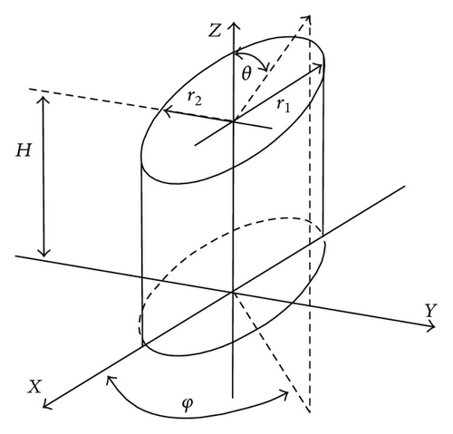
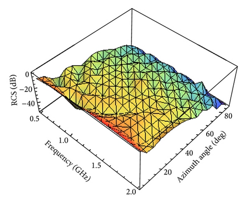
The LW-MBPE technique described in the above section was first applied to an elliptical cylinder (Figure 1) over a frequency range of 0.5–2 GHz. The symmetry of this problem may be investigated such that it is only necessary to use the interpolation over the limited range 0°θ ≤ 90°. The Padé rational function was chosen to have a numerator order n = 8 and a denominator order n = 7. The fitting frequencies selected were 0.5,0.6,0.7, …, 1.9 and 2 GHz. These conditions were used to construct a matrix of the form given in (11), where n + d + 1 = 16. The nonnormal incidence backscattered RCS for an elliptical cylinder due to a linearly polarized incident wave is given by [20]
()
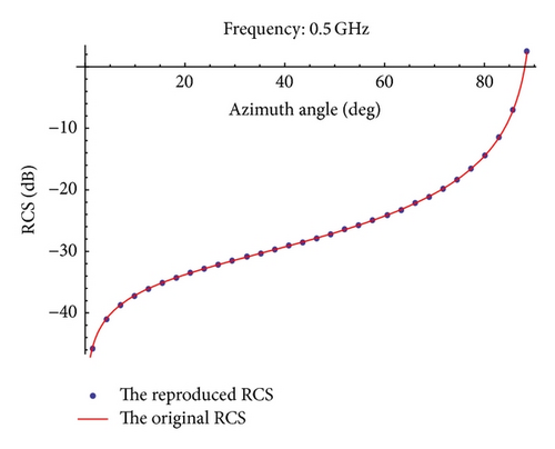
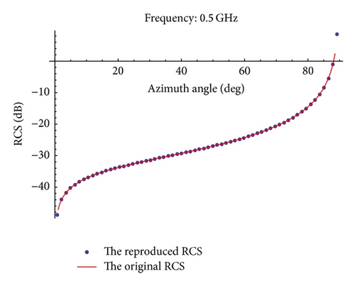
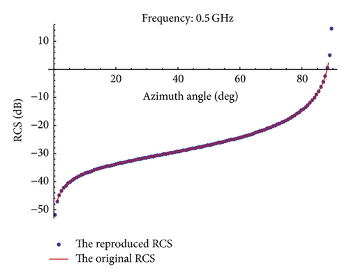
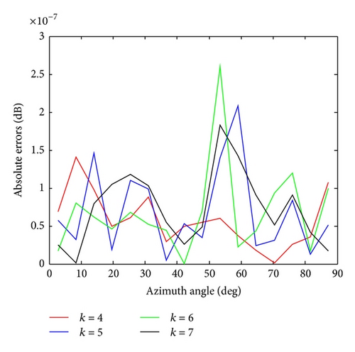
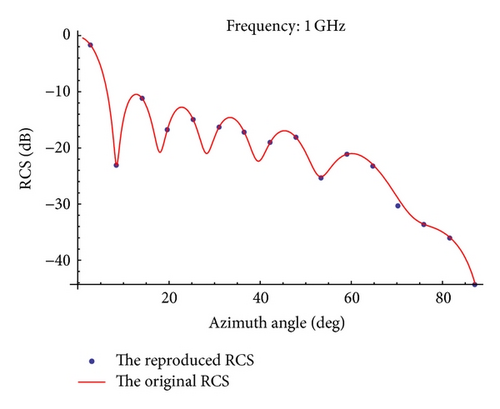
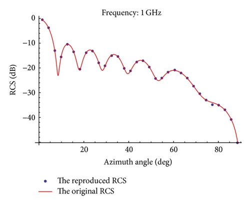
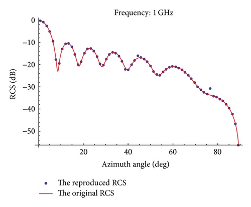
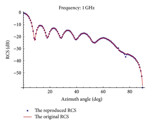
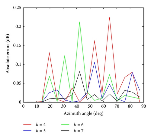
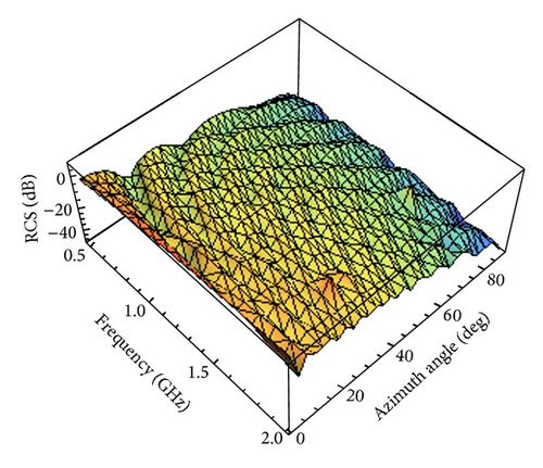
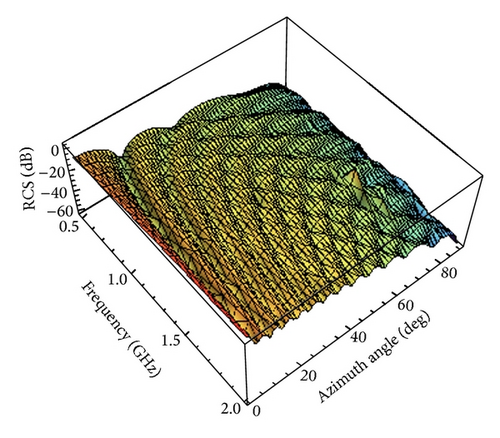
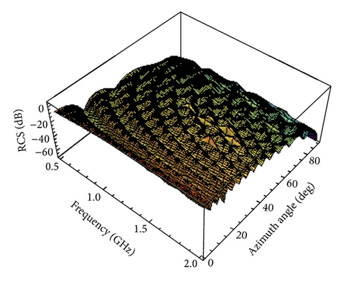
Figures 2, 3, 4, and 5 show the elliptical cylinder (r1 = 0.125 m, r2 = 0.05 m) backscattered RCS using (25) and the reproduced RCS using LW-MBPE method for different k, M = 2. The absolute errors for the reproduced RCS and original RCS in Figures 25 are shown in Figure 6. From Figure 6, we can find easily that the absolute errors are rather small.
Details are in the caption following the image
Elliptical cylinder.
Details are in the caption following the image
Backscattered RCS for an elliptical cylinder of k = 4 and φ = 45°.
Details are in the caption following the image
Backscattered RCS for an elliptical cylinder of k = 5 and φ = 45°.
Details are in the caption following the image
Backscattered RCS for an elliptical cylinder of k = 6 and φ = 45°.
Details are in the caption following the image
Backscattered RCS for an elliptical cylinder of k = 7 and φ = 45°.
Details are in the caption following the image
Absolute errors for different k and φ = 45°.

Table 1 shows the absolute errors between the original RCS and the reproduced RCS. From Table 1, we can also see that the errors are smaller and smaller when k increases.

Table 1. The absolute errors between original RCS and reproduced RCS for different k (dB).
θ × 90° k = 4 k = 5 k = 6 k = 7
0.1 0.00874 0.00540 0.00079 0.00035
0.2 0.02334 0.00354 0.00157 0.00019
0.3 0.03044 0.00348 0.00177 0.00024
0.4 0.02269 0.00924 0.00112 0.00055
0.5 0.25790 0.05183 0.01178 0.00281
0.6 0.03000 0.01726 0.00251 0.00113
0.7 0.11124 0.01937 0.00794 0.00097
0.8 0.32609 0.02837 0.01630 0.00237
0.9 6.49094 0.32208 0.02801 0.01609

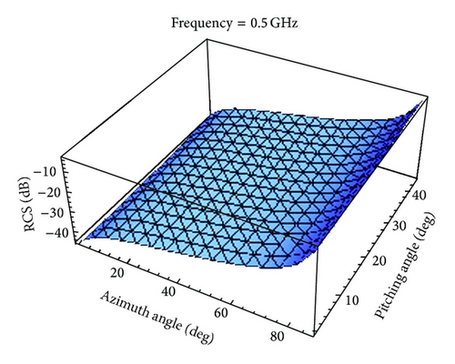
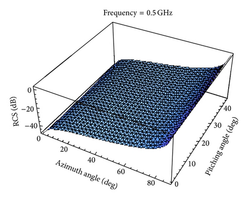
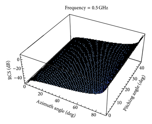
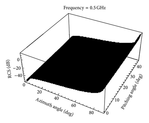
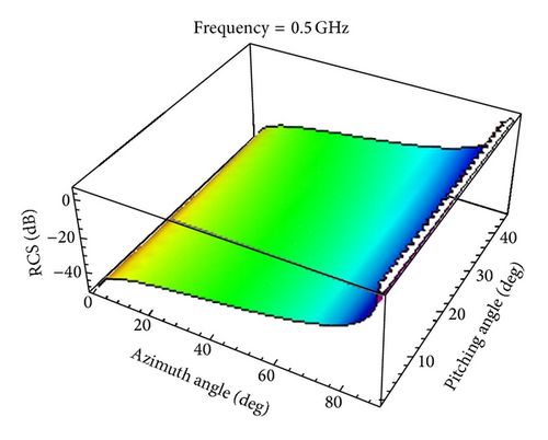
The interpolated RCS as a function of azimuth angle θ and pitching angle φ is shown in Figures 710 for . The elliptical cylinder backscattered RCS using (23) is also shown in Figure 11. Table 2 shows the absolute errors between the original RCS and the reproduced RCS for different values of θ, φ, and .

Table 2. The absolute errors between original RCS and reproduced RCS for different (dB).
(θ × 90°,   φ × 45°)
(0.1, 0.1) 0.01014 0.00610 0.00084 0.00041
(0.2, 0.2) 0.02629 0.00398 0.00176 0.00021
(0.3, 0.3) 0.03376 0.00383 0.00208 0.00031
(0.4, 0.4) 0.02468 0.01020 0.00132 0.00059
(0.5, 0.5) 0.27407 0.05570 0.01286 0.00302
(0.6, 0.6) 0.03233 0.01845 0.00270 0.00122
(0.7, 0.7) 0.11657 0.01995 0.00828 0.00102
(0.8, 0.8) 0.33268 0.02912 0.01669 0.00241
(0.9, 0.9) 6.49592 0.32396 0.02837 0.01616
Details are in the caption following the image
Backscattered RCS for an elliptical cylinder for θ, φ of .
Details are in the caption following the image
Backscattered RCS for an elliptical cylinder for θ, φ of .
Details are in the caption following the image
Backscattered RCS for an elliptical cylinder for θ, φ of .
Details are in the caption following the image
Backscattered RCS for an elliptical cylinder for θ, φ of .
Details are in the caption following the image
The elliptical cylinder backscattered RCS for θ, φ.

We can see that the reproduced RCS is more and more close to the original RCS with the value of becoming large by taking a closer look at Figures 711 and Table 2.

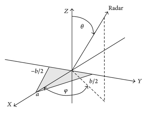
The second example used to demonstrate this new LW-MBPE procedure was a triangular flat defined by the isosceles triangle as oriented in Figure 12 (a = 0.2 m, b = 0.75 m). The RCS interpolation used the rational function with a numerator order n = 8 and a denominator order n = 7. The frequency domain sampling was done at sixteen frequencies (i.e., 0.5,0.6, …, 1.9 and 2 GHz). The backscattered RCS can be approximated for small aspect angles (less than 30°) by [20]
()
where α = kasin⁡θcos⁡φ, β = kbsin⁡θsin⁡φ, and A = ab/2.
Details are in the caption following the image
Coordinates for a perfectly conducting isosceles triangular flat plate.

Based on a perfectly conducting isosceles triangular flat plate, Figures 13, 14, 15, and 16 show the normalized backscattered RCS using (26) and the reproduced RCS using LW-MBPE for k = 4,5, 6,7. The absolute errors for the reproduced RCS and original RCS in Figures 1316 are shown in Figure 17.

Details are in the caption following the image
Backscattered RCS for a perfectly conducting triangular flat plate, k = 4 and φ = 60°.
Details are in the caption following the image
Backscattered RCS for a perfectly conducting triangular flat plate, k = 5 and φ = 60°.
Details are in the caption following the image
Backscattered RCS for a perfectly conducting triangular flat plate, k = 6 and φ = 60°.
Details are in the caption following the image
Backscattered RCS for a perfectly conducting triangular flat plate, k = 7 and φ = 60°.
Details are in the caption following the image
Absolute errors for different k and φ = 60°.

Table 3 shows the absolute errors between the original RCS and the reproduced RCS. From Table 3, we can also find that the errors are smaller and smaller with k increasing.

Table 3. The absolute errors between reproduced RCS and original RCS for different k (dB).
θ × 90° k = 4 k = 5 k = 6 k = 7
0.1 8.54737 5.98691 0.86121 0.56261
0.2 6.56903 1.79307 1.08659 0.14338
0.3 3.55198 0.15870 0.04182 0.01021
0.4 0.69205 0.03673 0.03452 0.00126
0.5 0.33927 0.10280 0.02992 0.01416
0.6 2.76694 0.71435 0.21953 0.00813
0.7 0.61607 0.03730 0.01911 0.00141
0.8 0.04907 0.01372 0.00938 0.00182
0.9 0.09652 0.07825 0.05342 0.04251

The interpolated RCS as a function of azimuth angle θ and frequency is shown in Figures 1821 for different .

Details are in the caption following the image
Backscattered RCS for a perfectly conducting triangular flat plate for θ and frequency of .
Details are in the caption following the image
Backscattered RCS for a perfectly conducting triangular flat plate for θ and frequency of .
Details are in the caption following the image
Backscattered RCS for a perfectly conducting triangular flat plate for θ and frequency of .
Details are in the caption following the image
Backscattered RCS for a perfectly conducting triangular flat plate for θ and frequency of .

According to the above analysis, we can acquire the approximate backscattered RCS of the perfectly conducting triangular flat plate for arbitrary θ and frequency by using LW-MBPE method. What is more, the approximations are more and more accurate with increasing. It is evident from the examples that the LW-MBPE method is convergent.

In the two examples, the approximate formulas of the target backscattered RCS are known. However, in practical, the majority of targets backscattered RCS are unknown, and approximate formulas cannot be found. We can also obtain the value of RCS of sampling points by using the method of moments (MoM).

5. Conclusion

In this paper, a scheme to interpolate target RCS in both the frequency and spatial domains simultaneously using LW-MBPE method was proposed. The Padé rational function fitting model used for MBPE in the frequency domain can be easily modified to include spatial dependence on its numerator and denominator coefficients. This interpolation technique was applied to two examples, an elliptical cylinder and a perfectly conducting triangular flat plate; in each case, the modified Padé rational function yielded excellent coincidence with the exact results calculated using their RCS formulas. The results also show that the proposed method is convergent with sampling points increasing.

Nomenclature

  • ψnm(x):
  • Legendre wavelets function
  • Pm(x):
  • Legendre polynomials
  • ci, uij:
  • Wavelets coefficients
  • F(s):
  • Padé rational function
  • :
  • Padé rational function coefficients
  • θ:
  • Azimuth angle
  • φ:
  • Pitching angle
  • σ:
  • Radar cross section
  • f:
  • Frequency
  • :
  • Positive integer
  • Pi:
  • Power density, or intensity, of a plane wave striking the target
  • Ps:
  • Power per unit solid angle reflected by the target.
  • Conflict of Interests

    There is no conflict of interests related to this paper.

    Acknowledgment

    This work was supported by the National Natural Science Foundation of China under Grant no. 51307004.

      Appendices

      A. The proof of Theorem 1

      Proof. Let F(θ, sl) be a function defined on [0,1] such that

      ()
      where is a positive constant.

      The orthonormality of sequence {ψnm(θ)} on [0,1) implies that , where I is the identity matrix; then

      ()
      where ; then we can get
      ()
      Now, let ; then
      ()
      Thus
      ()
      Therefore, we have
      ()
      Then we obtain
      ()
      namely,
      ()
      This completes the proof.

      B. The proof of Theorem 2

      Proof. The orthonormality of the sequence {ψi(θ)} on [0,1) implies that , where I is the identity matrix; then

      ()
      The Legendre wavelets coefficients of function F(θ, φ, sl) are defined by
      ()
      Let ; by change of and dθ = (1/2k)dt, we obtain
      ()
      Now, let τm(t) = (2m − 1)Pm+2(t) − 2(2m + 1)Pm(t)+(2m + 3)Pm−2(t); then we have
      ()
      By solving this equation, we have
      ()
      where A(k, m) = (1/25k+1(2m + 1))(1/(2m − 1) 2(2m + 3) 2).

      So we have

      ()
      Moreover, it was shown in the above equation that
      ()
      thus, we have
      ()
      Namely,
      ()
      Therefore, we have
      ()
      where is a constant.

      Then we get

      ()
      thus,
      ()
      This completes the proof.

        The full text of this article hosted at iucr.org is unavailable due to technical difficulties.