Volume 2015, Issue 1 379576
Research Article
Open Access

On the Stability and Equilibrium Points of Multistaged SI(n)R Epidemic Models

Raul Nistal

Raul Nistal

Institute of Research and Development of Processes, University of the Basque Country, Campus of Leioa, P.O. Box 644, Barrio Sarriena, Bilbao, Bizkaia, 48940 Leioa, Spain ehu.eus

Search for more papers by this author
Manuel de la Sen

Manuel de la Sen

Institute of Research and Development of Processes, University of the Basque Country, Campus of Leioa, P.O. Box 644, Barrio Sarriena, Bilbao, Bizkaia, 48940 Leioa, Spain ehu.eus

Search for more papers by this author
Santiago Alonso-Quesada

Santiago Alonso-Quesada

Institute of Research and Development of Processes, University of the Basque Country, Campus of Leioa, P.O. Box 644, Barrio Sarriena, Bilbao, Bizkaia, 48940 Leioa, Spain ehu.eus

Search for more papers by this author
Asier Ibeas

Corresponding Author

Asier Ibeas

Department of Telecommunications and Systems Engineering, Universitat Autònoma de Barcelona, Bellaterra, 08193 Barcelona, Spain uab.cat

Search for more papers by this author
Aitor J. Garrido

Aitor J. Garrido

School of Industrial Technical Engineering, University of the Basque Country, Paseo Rafael Moreno 3, 48013 Bilbao, Spain ehu.eus

Search for more papers by this author
First published: 14 May 2015
Citations: 12
Academic Editor: Qing-hua Ma

Abstract

This paper relies on the concept of next generation matrix defined ad hoc for a new proposed extended SEIR model referred to as SI(n)R-model to study its stability. The model includes n successive stages of infectious subpopulations, each one acting at the exposed subpopulation of the next infectious stage in a cascade global disposal where each infectious population acts as the exposed subpopulation of the next infectious stage. The model also has internal delays which characterize the time intervals of the coupling of the susceptible dynamics with the infectious populations of the various cascade infectious stages. Since the susceptible subpopulation is common, and then unique, to all the infectious stages, its coupled dynamic action on each of those stages is modeled with an increasing delay as the infectious stage index increases from 1 to n. The physical interpretation of the model is that the dynamics of the disease exhibits different stages in which the infectivity and the mortality rates vary as the individual numbers go through the process of recovery, each stage with a characteristic average time.

1. Introduction

There is a very relevant interest in the literature concerning different aspects of dynamics of populations and related biological modeling issues including their positivity, stability, controllability, and observability and appropriate design of control rules for such models. The interest is twofold; namely, (a) on the one hand they have an undoubted mathematical interest because of the rich nonlinear dynamics they can exhibit which makes its analysis nontrivial in most cases, (b) on the other hand they have relevant interests in the real world concerning aspects such as health, resource exploitation, or rationalization of the labor management force towards economical issues. Biological and population dynamics models are usually defined by a variety of mathematical tools. Among them we can find differential and difference equations, eventually including internal delayed dynamics (i.e., delays in the state) or external delays (i.e., delays in the forcing action, if any) [18]. The delays can be, in general, modeled as point delays or as distributed delays and as constant or as time-varying delays. The background literature on the various involved subjects is exhaustive. In that context, important interest has been devoted to models of interaction of species versus their habitat, such as, for instance, the various Beverton-Holt models and some related generalizations, with their intrinsic problems of positivity, equilibrium analysis, stability, oscillatory solutions, and their control; see, for instance, [9, 10] and references therein. Important attention is paid to the study of their inverse models and their control which are equivalent to the initial direct ones while being much more tractable mathematically [9, 10]. Control rules through the online design of the habitat carrying capacity have been dealt with and applied in aquaculture exploitation [9]. Logistic equations, predator-prey models, and related oscillatory regimes have been also studied in the background literature (see, e.g., [1113]). On the other hand, epidemic models of various kinds ranging from very elementary to sophisticated have received and still receive important attention. The literature is exhaustive (see, e.g., [18, 1435]). Basic models are named via acronyms as SIR (susceptible-infectious-removed by immunity), SEIR (susceptible-infected-infectious-removed by immunity), or SVEIR (susceptible-vaccinated-infected-infectious-removed-by-immunity) models according to the involved subpopulations with coupled dynamics. An alternative popular name for the infected population is “the exposed” (those without external symptoms but already incubating the disease). An alternative popular name for the removed-by-immunity population is “the immune." There are also a wide variety of extended models available built with combinations and extensions of the above ones. The main properties dealt with are the calculation and related stability analysis of the disease-free and endemic equilibria, the infection permanence, which leads to the impossibility of reaching the disease-free equilibrium, and the positivity of the trajectories whose analysis combined with the boundedness of the total population leads to the internal stability [2, 3, 18, 20, 22, 24] of the whole model implying the boundedness of all the subpopulations [25, 18, 20, 22, 2428, 30, 31, 35]. The control action on an epidemic model is performed through vaccination rules which can be of different types, for instance, constant or based either on linear or nonlinear feedback of some measurable or known subpopulations, mainly, the infectious population. Vaccination laws can also be of an impulsive nature (in practice, acting with large efforts along very short periods of time) or of a combined regular/impulsive nature [2, 57, 2631]. In particular, the technique of adaptive sampling to design the relevant vaccination time instants is combined with the design of vaccination rules in [30] so as to increase the vaccination performance towards the disease eradication. It has to be pointed out that epidemic models are essentially uncontrollable so that it is not possible to drive simultaneously via a vaccination rule all the subpopulations to prefixed arbitrary values in finite prefixed time intervals since the total population is a constrain for all time for the sum of all the subpopulations [2, 7, 26]. However, most of the models are output controllable, or at least output stabilizable, with the outputs being defined “ad hoc” by either the infected and/or infectious subpopulations or the susceptible plus the immune subpopulations, those defined to be the output of the dynamic system, if necessary. The relevant idea in the epidemic models is that there is a transfer in-between subpopulations along the infection process (being, therefore, uncontrollable). The agent transmitting the infection is a quadratic dynamics of the susceptible and infected population with some either constant or functional factors (the incidence rate) which depends on a parameter or functional factor (the coefficient transmission rate) which depends on each infectious disease and the population nature [3, 16]. There is a very basic parameter to analyze, called the basic reproduction number, which has the following two interpretations.
  • (a)

    If it ranges from zero to one, the disease-free equilibrium is asymptotically stable and the infection asymptotically vanishes without requiring any external action on the system. In this case, the Jacobian of the matrix of the dynamics of the epidemic model defining the linearized state-trajectory has all its eigenvalues in the stable region. If it exceeds one, the disease-free equilibrium is unstable so that the state trajectories can converge asymptotically to the endemic equilibrium or exhibit an oscillatory behavior.

  • (b)

    The infection cannot progress if the reproduction number is less than one since the minimum available initial infected population to propagate the disease is below its critical value for spreading.

However, the explicit expression of the reproduction number is neither direct nor easy to obtain in sophisticated epidemic models. Therefore, more advanced techniques, based on the so-called next generation matrix, have been proposed to define such a reproduction number; see, for instance, [8, 3335]. More recent studies on epidemic models are described in [36, 37]. The importance of demographics is taken into account in [36], while the stability of the equilibrium points of a delayed disease is described in [37]. This paper addresses the concept of the next generation matrix for a new proposed extended continuous time SEIR model referred to as SI(n)R model with delays where there are n-successive stages of infectious subpopulations, each one acting at the exposed subpopulation of the next infectious stage in a cascade global disposal. Since the susceptible subpopulation is common to all infectious stages, its impact on each of those stages is modeled with an increasing delay as the infectious stage index increases from 1 to n. A second related model is used without the above delay. Both models are also reformulated with discretized versions. The physical interpretation of the SI(n)R models is that the incubating period of any disease is not identical for all the susceptible individuals so that they can become infected at different times. So, each of the infectious stages is an infectious class which includes a certain number of individuals which become infected at times centered about a reference average time instant which is considered common for the whole group. The stability analysis is performed by defining a basic reproduction number from an ad hoc next generation matrix for this model. The basic properties which are proved are as follows. (1) All the trajectories remain bounded since the differential system is nonnegative, as it is the alternative discrete model, in the sense that all the subpopulations are nonnegative for all time, and the total population is uniformly bounded for all time. (2) If the defined basic reproduction number is less than one, then the disease-free equilibrium point is globally asymptotically stable as it is proved through the definition and use of a Lyapunov function. In this case, the endemic equilibrium point is locally unstable and, furthermore, it is unfeasible (i.e., nonreachable by any trajectory) since it is not compatible with the system positivity. (3) If such a basic reproduction number is equal to one, then the endemic equilibrium does not exist as such since it is identical to the disease-free equilibrium and then globally stable since the system is positive and the total population is uniformly bounded for all the time so that none of the subpopulation can be unbounded. (4) If the basic reproduction number exceeds one then the disease-free equilibrium point is locally unstable.

2. The Model

This section contains the description and main properties of the introduced models. Previous models of multistaged infectious diseases have been described in [38] including (a) the so-called epidemic models with multistaged infectious period where the susceptible population influences the first infectious stage, that one, the second infectious stage, and so on; (b) the epidemic models with several types of infective subpopulations which are influenced in a parallel disposal and all of them have transitions to a unique removed population; (c) the epidemic among a number of homogeneous groups (each susceptible group generates its own SIR model). It can be considered, in a general context, that the structure proposed in this paper lies in the first of the above classes of the multistaged models.

2.1. SI(n)R Model with No Delays

The proposed model is described as a succession of infectious stages of the disease, each one with a characteristic infectivity rate βi. The susceptible subpopulation goes through each infected subpopulation until they reach the recovered subpopulation, immune to the disease for a certain time until they become susceptible again. The susceptible population is born at a rate α while the death rate of each infectious subpopulation is νi = b + ξi, with b being the natural death rate of the population and ξi the mortality rate associated with the disease at each infectious stage. The transition rate from the ith infectious subpopulation to the next one as well as the transition rate from the last infectious subpopulation to the recovered one is denoted by γi, while the transition from the recovered to the susceptible is μ−1. All the parameters are assumed to be positive so as to possess full physical meaning. The equations for the dynamics of the subpopulations are coupled as follows:
(1)
where S and R are the susceptible and recovered subpopulations and Ii are the various infectious subpopulations corresponding to the different infection stages. For notation simplicity, the vector x is defined as
(2)

Now the positivity, existence of equilibrium points, and stability are studied for this model.

2.1.1. Positivity and Boundedness

Proposition 1. All the subpopulations remain nonnegative for all time for any given nonnegative initial conditions, xi ≥ 0  ∀ i ∈ [1, …, n + 2] and all t ≥ 0.

Proof. Let ts > 0 be so that S(ts) = 0 and R(ts), Ii(ts) ≥ 0  ∀ i ∈ [1, …, n]. Then, from 1

(3)

Now, let t1 > 0 be so that I1(t1) = 0 and S(t1), Ii(t1) ≥ 0  ∀ i ∈ [2, …, n]. Then, from 1

(4)

For the next (n − 1) infectious subpopulations the same operation is made: let tj > 0 be so that Ij(tj) = 0 and S(tj), Ii(tj) ≥ 0  ∀ ij. Then, from 1

(5)

Finally, let tr > 0 so that R(tr) = 0 and S(tr), Ii(tr) ≥ 0, ∀i ∈ [1, …, n]. Then, from 1

(6)
Since it has been proven that none of the subpopulations will have a negative derivative at any time instant when they vanish and the rest of the subpopulations are nonnegative, then all the subpopulations must have nonnegative values for all time.

Not only does the epidemic system possess nonnegative solutions under nonnegative initial conditions, but also the total population and all the subpopulations are bounded for all time with a uniform finite upper-bound as it is discussed in the subsequent two results.

Proposition 2. The total population is finitely upper-bounded for any given nonnegative initial conditions.

Proof. If we sum up 1, we obtain

(7)
Since Proposition 1 guarantees the nonnegativity of subpopulations and all the parameters are assumed to be positive, then as ξj ≥ 0 and Ij(t) ≥ 0 for all time t ≥ 0, for all t ≥ 0 and
(8)
The solution to the differential inequality 8 is given by
(9)
for all t ≥ 0. Thus, the total population is finitely upper-bounded and the proposition is proved.

Corollary 3. All the subpopulations are finitely upper-bounded for all time for any given nonnegative initial conditions, obeying the constraints , where is the total population at the disease-free equilibrium.

2.1.2. Equilibrium Points

The equilibrium points are obtained by zeroing the left-hand side of 1, resulting in
(10)
This system possesses in general two solutions. The first one is the disease-free equilibrium point (DFE) in which the infectious and recovered subpopulations vanish so that the susceptible becomes the total population :
(11)
and the endemic equilibrium point (END), described as
(12)
is . Note that if , then , so the endemic equilibrium is not feasible so that the only reachable equilibrium point is the disease-free equilibrium point. In the next section, it is seen that this situation corresponds to the reproductive number R0 to be less than one. Once we have the expressions of both equilibrium points, we are prepared to discuss their equilibrium in the next section.

2.1.3. Stability Analysis: Next Generation Matrix

The local stability of the DFE point is proved in this section after introducing the reproductive number R0, which is the average number of new cases that produce an infected individual during the average duration of the disease. In order to find this number easily, a next generation matrix with small domain is constructed as follows. The Jacobi matrix defined around the disease-free equilibrium is composed of four different submatrices: F, Σ, A, and C:
(13)
where
(14)
would be the transmission matrix, representing the appearance of new infections, while
(15)
represent the remaining transitions of the infected subpopulation unrelated as the deaths, or the transition from recovered to susceptible. Then, the inverse of that matrix Σ−1 would represent the average time in which a subpopulation stays in an infected state. The next generation matrix will be then defined as K = −FΣ−1, and the reproductive number R0 corresponds to the spectral radius of K. Thus, the spectral radius is given by
(16)
Thus, the stability of the disease-free equilibrium point is directly related to this spectral radius. In this way, it will be locally asymptotically stable when R0 < 1, while R0 > 1 will imply instability of such a DFE point [35]. Studies of epidemic models with a parallel disposal of several submodels of susceptible-infectious-recovered subpopulations have proven that, for R0 > 1, the endemic point is locally asymptotically stable [39]. Remember that it has been proven in previous section, 12, that if R0 < 1, the only reachable point is the disease-free equilibrium, which is also locally asymptotically stable. If R0 = 1, both equilibrium points coincide (see 12).

2.2. Discrete SI(n)R Model with No Delays

This section considers the discrete-time counterpart of the continuous-time model 1. In the discrete framework notation the subpopulations are written as for any time t ∈ [kτ, (k + 1)τ. The discrete model will be based on the continuous one from 1, with a step size τ > 0. Thus, it is defined as the change , with as in the continuous subpopulations from 2. Therefore, it is obtained for k ≥ 1 that
(17)

Proposition 4. The discrete system described in 17 is nonnegative for any nonnegative initial conditions if the step size τ is small enough to satisfy

(18)
with , , and , where βM = max⁡1≤jn⁡[βj] and N1 is the total initial population (i.e., the total population at the initial time).

Proof. Given a set of nonnegative subpopulations at the kth-sample, from the second equation of 17, it can be deduced that

(19)
Then, Rk+1 ≥ 0 if ττ2. The same method can be applied for guaranteeing the nonnegativity of . From the third and fourth equations at 17, it is deduced that
(20)
Then, if τ ≤ min⁡1≤mn⁡[τm+2].

In order to guarantee the nonnegativity of the susceptible subpopulation, first a maximum value is set for Nk. From 17

(21)
then ∀k ≥ 1, and it can be said that
(22)

So from the first equation at 17 it is known that

(23)
Then, given that , j > 0, it is defined that τ1 = 1/(b + βM(N1 + α/b)) so that the susceptible subpopulation remains nonnegative if
(24)
Thus, for a step size τ ≤ min⁡⁡[τ1, τ2, τ3, …, τm], the system remains positive.

The equilibrium points are obtained by making xk+1 = xk = x* in 17:
(25)
The solutions of the above system of equations are the same as in the continuous-time case and given by 11 and 12 for the disease-free and endemic equilibrium points, respectively. A next generation matrix approach for discrete models is made so that the Jacobian matrix evaluated at the disease-free equilibrium is as follows:
(26)
The Jacobian takes the form
(27)
The Jacobian can be separated into four submatrices as follows:
(28)
with the fertility submatrix n × n, related to the new infections and represented as F and the transition submatrix Σ, with the same dimensions, related to the transition of the individuals between the different subpopulations resulting in
(29)
A simple calculation with the Jacobian matrix results in an equivalent decomposition of the whole linearization about the equilibrium system into two complete subsystems, one describing the infection progress while the other one expresses the disease-free subpopulation dynamics as follows:
(30)
The term Σi,j represents the fraction of the individuals from the jth infected subpopulation that will survive and move to the ith. Because of these demographic interpretations, from Perron-Frobenius theory on the maximum modulus [40], the parameters are set so that the column sum of Σ and the maximum moduli of its eigenvalues are less than one; that is, ρ[Σ] < 1, so as to exclude the case of an immortal population. Then, it can be established for the vector of initial infectious individuals that lim⁡k⁡(−Σ)ky0 = 0. Then, the next generation matrix Q can be defined as the sum of the infections ever produced by the infected individuals at tk for all the time they remain infectious, which would be Fyk at tk, −FΣyk at tk+1, and FΣ2yk at tk+2 ad infinitum:
(31)
where Q represents the distribution of all infections accumulated during the lifespan of the infectious population:
(32)
Then the basic reproduction number is defined as the spectral radius of the Q matrix R0 = ρ[Q] = ρ[F(I + Σ)−1]. The spectral radius of the FΣ is defined as ρ[FΣ] = r. It is proven in [40] that either r = R0 = 1 or 1 < r < R0 or 1 > r > R0 > 0, so the stability of the disease-free equilibrium is determined by the value of R0. In our model this reproduction number is obtained as
(33)

Thus, the disease-free equilibrium state will be locally stable when the reproduction number is less than 1 and unstable otherwise. From known previous calculations of the stability of similar models [35, 40], this decomposition technique for stability analysis can be compared to previous ones such as the study of the stability made in [35] for the SEIR model, which is a specific version of a continuous SI(n)R model in which n = 2  β1 = 0, ν1 = ν2 = b, and γ1 = κ. From the definition in 33 it is obtained that R0 = β2Sdfeκ/(b + κ)(b + γ2), which agrees with the study of the eigenvalues of the Jacobian in a continuous-time model [26].

2.3. SI(n)R Model with Delays

2.3.1. Construction of the Model

A new model is proposed based on the previous one in which the transition rates between subpopulations are substituted by delays, implying that each individual must stay at each stage of the infection during a certain period of time (latent period) before recovery. Such time periods are defined as for the infectious stages of the disease and τR = μ for the recovered state. The model also preserves the infectivity mechanism of the previous one, in which all the infectious subpopulations affect the infection of the first stage at different rates. For notational abbreviation in the subsequent exposition it is now defined as the function . Thus, the value of the infected subpopulation I1 at a certain time t is defined by the ratio of the people that became infected at time ω < t that has not passed to the I2 infectious subpopulation yet. In order to calculate such a total amount, consider the probability
(34)
with ρ1(ξ) being the probability distribution of the transition I1I2 plus the probability to stay alive after time tω, which would be equal to . An integration ω ∈ (−, t) is made in order to obtain the value of the subpopulation at the instant t resulting in
(35)
Given the above integral function of the first stage of the infectious subpopulations, its derivative through time is easily obtained as
(36)
The probability distribution of transition is defined as ρ1(ω) = δ(ωτ1), meaning that the probability of transition of the subpopulation at the stage 1 of the disease to the next one is set to zero before it has passed a latent time interval τ1 and is equal to 1 after that time, so that 36 transforms to
(37)
As the rate of death in the subpopulation I1(t) corresponds to −ν1I1(t), it is inferred that the term corresponds to the rate of transition from I1(t) to I2(t). Then, the value of the people that arrives at I2 at ω < t would be , and I2 at certain time would be written as . For any subpopulation m ∈ [1,2, …, n], it can be written that
(38)
For the recovered subpopulation the same technique is used, so that the dynamic of R over time can be written as
(39)
with , , and , Tn+1 = Tn + τR. The dynamic equations of the subpopulations are defined then as
(40)
where, as in the previous model, α is the constant birth rate, and the fully immune recovered subpopulation eventually becomes susceptible again after the period of time τR.

2.3.2. Positivity and Boundedness

Proposition 5. The model equation 40 is nonnegative for any initial nonnegative conditions. Thus,

(41)
ω ∈ (−, t0), which implies xi(t) ≥ 0; ∀m = 1,2, …, n + 2  ∀ t ∈ [t0,).

Proof. Since βi ≥ 0, it is then deduced from 41 that f(ω) ≥ 0  ∀ ω ∈ (−, t0). Assume that

(42)
then, from 40 at the time t0 + λ,
(43)
therefore, the subpopulation S will not be the first subpopulation to be negative.

From 38 assume that ∃t1t0 such that Im(t1) = 0 for the first time and the value ζ ≥ 0 as small as desired such that I(t1ζ) > 0; I(t1 + ζ) < 0. Then it can be said that

(44)

Since f(t1ζ) ≥ 0 and knowing that f(t) is continuous and derivable for all t, from the mean value theorem, it can be deduced that

(45)
which is in direct contradiction with the original assumption of I(t1ζ) > 0; I(t1 + ζ) < 0. Then as S(ω) is not negative before t1 ≥ 0, the term f(ω) will remain nonnegative. Consider ∀ω ∈ (−, t1 + ζ+). Therefore, neither the infectious nor the susceptible subpopulation will be the first one to have a negative value. The same method can be applied to demonstrate that the recovered subpopulation will not be the first to have a negative value either. Then, xi(t) ≥ 0  ∀ i = [1, …, n + 2] holds for all time for any given nonnegative initial conditions.

Since the lower bound of the subpopulations is established as 0, an upper-bound for all the subpopulations is set in the following proposition.

Proposition 6. S(t) ≤ Ndfe, Im(t) ≤ Ndfe, R(t) ≤ Ndfe  , for any given initial conditions .

Proof. The dynamic of N(t) is obtained from 40: . As νib  ∀ i = [1,2, …, n], and given the previous boundary of nonnegativity from Proposition 4, it can be seen that, for any t0N(t0) = α/b, . Thus, N(t) ≤ α/b  ∀ t > t0. Then, for each subpopulation

(46)
it is established that ; ∀t > t0.

2.3.3. Equilibrium Points

The existence of equilibrium points in our model is now studied. The dynamics of the subpopulation described in 40 is zero at the equilibrium points, so that
(47)
being . Two equilibrium points are obtained and result in
(48)
(49)
with ηj = (Cj−1Cj)/νj and . Note that 1 ≥ C1C2 ≥ ⋯≥Ci−1Ci ≥ ⋯≥Cn+1 ≥ 0 and νj ≥ 0  ∀ j, so ηj ≥ 0  ∀ j. Given any nonnegative initial conditions, the endemic equilibrium point would not be reachable if , as Γ and would be <0.

Take into account that if S* = α/b, xend = xdfe, the endemic, and the disease-free equilibrium are the same, so there is only one equilibrium point in the system.

2.3.4. Stability of the Disease-Free Equilibrium (DFE) Point

The local stability of the DFE point is proved in this section after introducing the reproductive number R0, the average number of new cases that produce an infected individual during the average duration of the disease. In order to find this number easily, a next generation is constructed as follows.

First, the vector of the subpopulations is reorganized as in 2, so that the Jacobian matrix around the DFE point can be properly written as
(50)
where F is the transmission matrix, representing the appearance of new infections Fij = Ci−1βj, while Σ represent the remaining transitions of the subpopulation which are unrelated directly to the infection, such as the deaths, or the transition from recovered subpopulation to susceptible subpopulation.
Then, the next generation matrix is given by K = −FΣ−1. The submatrices composing the Jacobian are
(51)
so the transmission and transition matrices are
(52)
i, j = 1, …, n. The element Kij is the number of new cases generated in the stage of the disease i by one infected case that has just arrived to the stage of the disease j. Then, the dominant eigenvalue of the next generation matrix K would correspond to the reproduction number R0. However, it is possible in this case to construct a small domain next generation matrix [35] KS with a lower dimension than K, from which it will be much easier to obtain this dominant eigenvalue. Since (a) R is a matrix whose rows are linearly independent vectors spanning the rows of F and (b) C is a matrix whose columns are linearly independent vectors spanning the columns of F, then F = CR, and the small domain next generation matrix will be defined as KS = −RΣ−1C. In our case and R = (β1, β2, …, βn), so
(53)
since dim⁡(KS) = 1, the dominant eigenvalue of KS would be KS. Note that KS = R0 implies that if R0≶1, then , which is also the condition of reachability of the endemic equilibrium, as stated in the previous section.

Proposition 7. The DFE is globally asymptotically stable if R0 < 1.

Proof. A candidate for a Lyapunov function Φ is defined as Φ = ϕ1 + ϕ2 + ϕ3, having the auxiliary functions ϕ1, ϕ2, ϕ3 been defined as

(54)
now, ϕ3 is positive definite ∀t, since f(ω) ≥ 0  ∀ ω, βi ≥ 0, bi > 0, and . To verify the positivity of ϕ1 + ϕ2, consider the definition of the infectious subpopulation from 38 and the probability transition function ρi(ξ) = δ(ξτi). It is then established that
(55)

This integral function can be reconfigured as

(56)

Given this definition of Ii(t), the parameter σi(t) is defined as

(57)
Since f(ω) ≥ 0 and , it is deduced that σi(t) ≥ 0  ∀ t, ∀i ∈ [1, …, n]. Then and ϕ3(t) ≥ 0  ∀ t. Thus the nonnegativity of the Φ function is proven. The function Φ is equal to zero for Ii(ω) = 0  ∀ i = 1, …, n, ∀ω ∈ [tTn, t]. Then the derivative over time is calculated as
(58)
. For R0 < 1 → S* > α/bS(t), so for Ii = 0  ∀ i = 1, …, n and otherwise from 40. Thus the proposition is proved.

2.3.5. Stability of the Endemic Equilibrium Point (END) Model with n = 1

For simple models, that is, models with only one or two infectious subpopulations, a study of the stability of their endemic points is also made. The model is linearized around the endemic point and the eigenvalues of the Jacobi matrix are obtained. The function f(λ) is defined as
(59)
with J the 3 × 3 Jacobi matrix from 40, defined at the endemic equilibrium point from 49:
(60)
The solutions of are
(61)
respectively, with and . Since b > 0 and , λ1 and λ2 are defined as negative. The third solution will be defined as negative λ3 < 0 if , which is satisfied for or, as is shown in Section 2.3.4, when R0 > 1.

2.3.6. Stability of the Endemic Equilibrium Point (END) Model with n = 2

For n = 2 (i.e., there are two infectious subpopulations) a function g(λ) will be defined as in 59, this time with J a 4 × 4 Jacobi matrix from the susceptible, the recovered, and the two stages of the infectious subpopulations:
(62)
with
(63)
being X = ν1ν2(β1(1 − C1) + β2(C1C2))/(β1(1 − C1)ν2 + β2(C1C2))ν1. The first eigenvalue is trivially obtained as λ = −b. The other eigenvalues will not be directly obtained, as it is only needed to demonstrate that their real part is negative in order to prove the local asymptotic stability of the model. The Routh-Hurwitz criterion [41] says that in order to have all the solutions of g(λi) = 0 on the left half plane, the coefficients of g must satisfy the following conditions:
  • (1)

    gi > 0  ∀ i = 0,1, 2,3

  • (2)

    g1g2 > g3g0.

Both conditions can be satisfied once that the limits of the X parameter are established. Given νM = max⁡[ν1, ν2] and νm = min⁡[ν1, ν2] then
(64)
so that, for , it is deduced that the coefficients are positive:
(65)
And the lower limit of the second condition is defined as
(66)
so all the real parts of the eigenvalues are negative and the equilibrium endemic point is locally asymptotically stable as long as R0 > 1.

2.4. Discrete SI(n)R Model with Delay

The dynamic equation 40 is approximated to , with being the vector of the subpopulations to obtain a discrete-time counterpart of the continuous-time model. The notation for any subpopulation at the time interval t ∈ [kτ, (k + 1)τ is established then as . Thus, the analogous discrete equations to the model from 17 are obtained:
(67)
and , σμ = σn + τμ, with and being Ni and Nμ the rounded half down value for τi/τ,  τμ/τ, respectively. Now, at the equilibrium point, the delays are not relevant, while the dynamic equation at the equilibrium can be rewritten as
(68)
The reproductive number will be obtained again with a next generation matrix method as in the previous section, so the value would be
(69)
which is similar to the reproductive number from the continuous model, with the only difference of the Di constants instead of the previous Ci. However, given their similar origins and values, the properties exhibited in both sets of constants will be the same, in the sense that 0 ≤ CnCn−1 ≤ ⋯≤C1 ≤ 1 such as 0 ≤ DnDn−1 ≤ ⋯≤D1 ≤ 1. Given the same SI(n)R model with the same characteristics, the values of the reproduction number will be very similar too.

3. Simulation

A set of Matlab simulations are made based on the models described in the previous section, in order to contrast the predictions on their respective endemic and disease-free equilibrium states. A large enough number of infectious subpopulations are chosen, n = 3, so the stability of the models will be tested regarding their reproductive numbers. A common initial condition is set to all the susceptible subpopulation in the disease-free equilibrium plus a 0.1 of that value of infected subpopulation at the first stage of the disease. For exposition and calculations convenience, the mortality rate b and the birth rate α will be both taken as equal to the inverse of the average lifespan of a human b = α = (1/70) year−1. The mortality rate of the three stages of the infection will be ν1 = 2b, ν2 = 3b, ν3 = 3b/2, and the average time which an individual spends in each stage will be 19, 29, and 61 days, respectively. The infectious ratios βi will be altered in order to obtain reproductive numbers below and above 1, but the ratios between them will be constant, as 4β1 = 7β2 = 4β3. When simulating the discrete models, an appropriate time step size is chosen in order to guarantee the nonnegativity of model with no delays. As for the discrete model with delays, given that nonnegativity of the subpopulations in the continuous model has been proved in Proposition 5, an algorithm is established during the simulation so that the discrete dynamics approximates to the continuous one in any critical positivity points. A loop in which the following point is evaluated is introduced, acting over the time step size. While any of the subpopulations of the next point present a negativity xk+1,i < 0 for any i ∈ [1, …, n + 2], then the step size is reduced , with j being the jth loop iteration, , and λ ∈ (0,1). Another loop is set after this resetting the time step size while the next point is nonnegative or the time step size is equal to or below the original value.

3.1. SI(3)R Model with No Delays

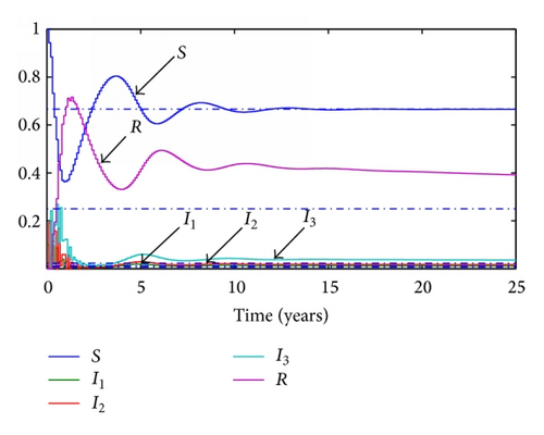
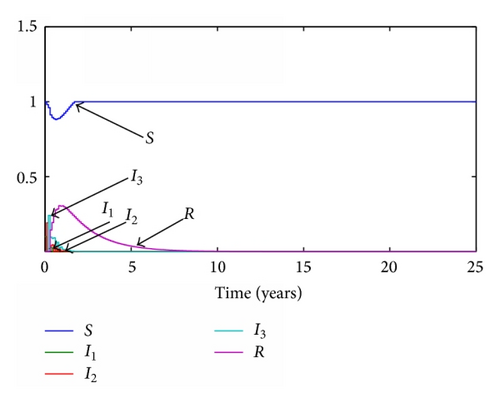
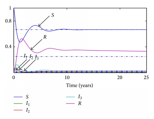
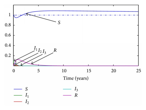
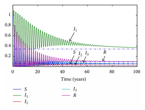
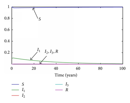
Given the parameters previously commented, the transition ratios between the different subpopulations are obtained as the inverse of their average times during each stage. Thus, γ1 = 365/19 year−1, γ2 = 365/29 year−1, γ3 = 365/61 year−1, and the final transition from recovered to susceptible again will be set as γ4 = 365/670 year−1. Given a value of the transition rates the reproduction number will be set to 0.5 and 1.5, respectively. For the continuous model, two graphics representing the evolution of each subpopulation for both situations are presented in Figures 1 and 2 while, for the discrete model, a step time τ is set to 0.1 years and the simulations are run with the same parameters. The results of these simulations are presented in Figures 3 and 4.
Details are in the caption following the image
Dynamic of the subpopulations for R0 = 1.5. The dotted lines represent the predicted endemic values.
Details are in the caption following the image
Dynamic of the subpopulations for R0 = 0.5. The dotted line represents the predicted disease-free value of the susceptible subpopulation.
Details are in the caption following the image
Dynamic of the subpopulations for R0 = 1.5. The dotted lines represent the predicted endemic values.
Details are in the caption following the image
Dynamic of the subpopulations for R0 = 0.5.

3.2. SI(3)R Model with Delays

The common parameters are set as in the previous cases, but this time the delayed times will be equal to their respective average times τ1 = 19/365 years, τ2 = 29/365 years, and τ3 = 61/365 years. The delay of the transition between the recovered and the susceptible subpopulations will be changed from 610/365 to 80/365 years in order to let the simulation achieve the simulation at a reasonable time. The values of the transmission rates will maintain their proportionality, but the range of the possible reproductive number is not so wide as in the previous case. Their values are changed to now be R0 = 1.01 and R0 = 0.92, respectively. The evolution of the subpopulations is presented in Figures 5 and 6.
Details are in the caption following the image
Dynamics of the SI(3)R model of the subpopulations for R0 = 1.01. The dotted lines represent the predicted endemic values.
Details are in the caption following the image
Dynamics model of the subpopulations of the SI(3)R for R0 = 0.92. Observe that the subpopulations rapidly tend to the disease-free equilibrium.

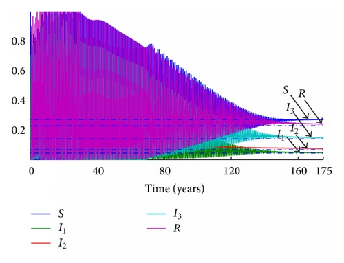
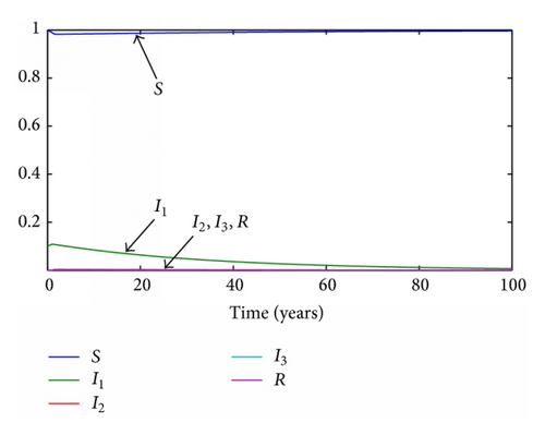
In the discrete model, the same time step as before is set to τ = 0.1 years. The evolution of the subpopulations for each reproductive number can be seen in Figures 7 and 8, respectively.
Details are in the caption following the image
Dynamics of the different subpopulations of the discrete delayed SI(3)R model for R0 = 1.01. The dotted lines represent the predicted endemic values.
Details are in the caption following the image
Dynamics of the subpopulations of the SI(3)R discrete delayed model for R0 = 0.92.

Observe that the subpopulations rapidly tend to the disease-free equilibrium in Figure 8. While it is seen that the discrete-time and continuous-time models reach the same final states when the conditions are equal, the irregularity of the dynamics in the discrete models over the continuous has also been noticed. This fact reveals that the discretization procedure along with the time step must be selected carefully prior to simulating the discrete-time model.

4. Conclusions

A model of a disease spreading with multiple infectious stages has been studied in depth. The next generation techniques have been proven to be quite useful when operating with models with complex interactions as in the variations of the model presented in this work. The reproduction numbers obtained in each case have also proven to predict correctly the final stable state of the subpopulations when they are properly simulated. The simulations have also shown that the different discretizations of a continuous model can cause significant discrepancies in the resulting dynamics. An appropriate integration step should be considered taking this into account as well as other factors like the computation time available, or, if the model is being used in a controlled system, the available time for data acquisition.

Conflict of Interests

The authors declare that there is no conflict of interests regarding the publication of this paper.

Acknowledgments

This work was partially supported by the Spanish Ministry of Economy and Competitiveness through Grant no. DPI2012-30651, the Scholarship support BES-2010-035160 for Raul Nistal, the Basque Government, through Grant no. IE378-10, and by the University of the Basque Country through Grant nos. UFI 11/07, PES13/21, and GIU14/07. Raul Nistal is grateful to the doctorate program “Molecular biology and Biomedicine” of UPV/EHU for its support for him as a Ph.D. student. Finally, the authors are also grateful to the reviewers for their useful suggestions.

      The full text of this article hosted at iucr.org is unavailable due to technical difficulties.