The problem of data recovery in multiway arrays (i.e., tensors) arises in many fields such as computer vision, image processing, and traffic data analysis. In this paper, we propose a scalable and fast algorithm for recovering a low-n-rank tensor with an unknown fraction of its entries being arbitrarily corrupted. In the new algorithm, the tensor recovery problem is formulated as a mixture convex multilinear Robust Principal Component Analysis (RPCA) optimization problem by minimizing a sum of the nuclear norm and the ℓ₁-norm. The problem is well structured in both the objective function and constraints. We apply augmented Lagrange multiplier method which can make use of the good structure for efficiently solving this problem. In the experiments, the algorithm is compared with the state-of-art algorithm both on synthetic data and real data including traffic data, image data, and video data.

1. Introduction

A tensor is a multidimensional array. It is the higher-order generalization of vector and matrix, which has many applications in information sciences, computer vision, graph analysis [1], and traffic data analysis [2–4]. In the real world, as the size and the amount of redundancy of the data increase fast and nearly all of the existing high-dimensional real world data either have the natural form of tensor (e.g., multichannel images) or can be grouped into the form of tensor (e.g., tensor face [5], traffic data tensor model [2–4], and videos), challenges come up in many scientific areas when someone confronts with the high-dimensional real world data. Because of some reasons, one wants to capture the underlying low-dimensional structure of the tensor data or seeks to detect the irregular sparse patterns of the tensor data, such as image compression [6], foreground segmentation [7], saliency detection [8], and traffic data completion [2, 3]. As a consequence, it is desirable to develop algorithms that can capture the low-dimensional structure or the irregular sparse patterns in the high-dimensional tensor data.

In the two-dimensional case, that is, the matrix case, the “rank” and “sparsity” are the most useful tools for matrix-valued data analysis. Chandrasekaran et al. [9] proposed the concept of “rank-sparse incoherence” to depict the fundamental identifiability of recovering the low-rank and sparse components. Wright et al. [10] and Candes et al. [11] demonstrated that if the irregular sparse matrix S is sufficiently sparse (relative to the rank of L), one can accomplish the sparse and low-rank recovery by solving the following convex optimization problem:

()

where A ∈ ℝ^m×n is the given matrix to be recovered; L ∈ ℝ^m×n is the low-rank component of A; S ∈ ℝ^m×n is the sparse component of A; ∥·∥_* denotes the nuclear norm defined by the sum of all singular values; ∥·∥₁ denotes the sum of the absolute values of matrix entries; μ is a positive weighted parameter. This optimization method is called the Robust Principal Component Analysis [10, 11] (RPCA) or the Principal Component Pursuit (PCP) due to its ability of exactly recovering the underlying low-rank matrix even in the presence of being corrupted by large entries or outliers.

Although the low-rank matrix recovery problem has been well studied, there is not much work on tensors. Li et al. [12] derived a method for the optimal Rank − (R₁, R₂, R₃) tensor decomposition model. Considering a real n-mode tensor

, the best Rank − (R₁, R₂, R₃) approximation is to find a tensor

with prespecified rank⁡_k(A_(k)) = R_k that minimizes the least-squares cost function:

()

The n-rank conditions imply that 𝒜^* should have the Tucker decomposition [13] as

. For the application, they applied the model to the high-dimensional tensor-like visual data by dividing the observed tensor into a low-dimensional structure plus unbounded but sparse irregular patterns: 𝒜 = ℒ + 𝒮. By assumption that the n-rank of ℒ should be small and the corruption 𝒮 is bounded, the original function is as follows:

()

In order to solve the problem, they made some conversions to (3) and extended the matrix robust PCA problem to the tensor case. A relaxation technique was used to separate the dependant relationships and the block coordinate descent (BCD) method was used to solve the low-n-rank tensor recovery problem. Then they proposed the rank sparsity tensor decomposition (RSTD) algorithm. In fact, their algorithm can be seen as a basic version of Lagrange multiplier method. Although being simple and provably correct, the RSTD algorithm requires a very large number of iterations to converge and it is difficult to choose the parameters for speedup. Besides, due to the property of the basic Lagrange multiplier method, the accuracy of results needs to be improved.

In this paper, a new algorithm for low-n-tensor recovery, which is termed as Mixture Augmented Lagrange Multiplier Method for Tensor Recovery (MALM-TR), is proposed. In the new algorithm, analogy to the RSTD [12], we convert the tensor recovery problem into a mixture convex optimization problem by adopting the relaxation technique strategy which eliminates the interdependent trace norm and ℓ₁ norm constrain. Actually, the elements involved in problem are all in matrix case. Thus, it can be treated as a multilinear extension of the RPCA problem and subsumes the matrix RPCA problem as a special case. Lin et al. [14] have proved that the matrix RPCA problem can be solved by ALM with achieving higher precision, being less storage/memory demanding, and having a pleasing Q-linear convergence speed. Inspired by these merits of ALM, we try to extend the augmented Lagrange multiplier method (ALM) to the multilinear RPCA problem and prove that ALM is not only fit to solve the matrix RPCA problem but also suitable to solve the multilinear RPCA problem.

For the usage of this algorithm, it is applied to real world data recovery including traffic data recovery, image restoration, and background modeling.

In traffic data analysis area, due to detector and communication malfunctions, traffic data often confronts with the noising data phenomenon, especially the outlier value noise, which has a great impact on the performance of Intelligent Transportation System (ITS). Therefore, it is essential to solve the issues caused by outlier data in order to fully explore the applicability of the data and realize the ITS applications. In the application part of this paper, we introduce the tensor form to model the traffic data, which can encode the multimode (e.g., week, day, record) correlations of the traffic data simultaneously and preserve the multiway nature of traffic data. For example, it is assumed that a loop detector collects traffic volume data every 15 minutes. Thus, it will have 96 records in a day. If we have 20 weeks traffic volume data, these data can be formed into a tensor of size 20 × 7 × 96. Then, the proposed tensor-based method which can well mine the multimode correlations of traffic data mentioned above is used to remove outlier noise of the traffic data.

It is observed that the multichannel image can be seen as a tensor with multidimensions. For example, RGB image has three channels including Red channel, Green channel, and Black channel. Thus, it can be represented as width × height × 3 which is a 3-dimensional tensor. For the application, the proposed method is used to remove the noise of the image. Though the method would not be reasonable for some natural images, it has many applications for visual data such as structured images (e.g., the façade image), CT/MRI data, and multispectral image. Besides images, video data can be grouped into the form of tensor. For example, there is a video which has 300 gray frames and each of which is in size of 200 × 200. These video data can form a tensor of size 200 × 200 × 300. For the video application, the proposed method will be used for background modeling.

The rest of the paper is organized as follows. Section 2 presents some notations and states some basic properties of tensors. Section 3 discusses the detailed process of our proposed algorithm. Section 4 tests the algorithm on different settings, varying from simulated data to applications in computer vision, image processing, and traffic recovery. Finally, some concluding remarks are provided in Section 5.

2. Notation and Basics on Tensor Model

In this paper, the nomenclatures and the notations in [1, 12] on tensors are partially adopted. Scalars are denoted by lowercase letters (a, b, c,…), vectors by bold lowercase letters (a, b, c,…), and matrices by uppercase letters (A, B, C,…). Tensors are written as calligraphic letters (𝒜, ℬ, 𝒞, …). N-mode tensors are denoted as

. The elements of an N-mode are denoted as

, where 1 ≤ i_k ≤ I_K, 1 ≤ K ≤ N. The mode-n unfolding (also called matricization or flattening) of a tensor

is defined as unfold(𝒜, n) = A_(n). The tensor element (i₁, i₂, …, i_N) is mapped to the matrix element (i_n, j), where

()

Therefore, , where . Accordingly, its inverse operator fold can be defined as fold(A_(n), n) = 𝒜.

The n-rank of a N-dimensional tensor

, denoted by r_n, is the rank of the mode-n unfolding matrix A_(n):

()

If the n-rank is very small related to the size of the tensor, we call it low-n-rank tensor.

The inner product of two same-size tensors

is defined as the sum of the products of their entries, that is,

()

The corresponding Frobenius norm is . Besides, the ℓ₀ norm of a tensor 𝒜, denoted by ∥𝒜∥₀, is the number of nonzero elements in 𝒜 and the ℓ₁ norm is defined as . It is clear that , and for any 1 ≤ n ≤ N.

The n-mode (matrix) product of a tensor

with a matrix

is denoted by 𝒜×_n M and is of size I₁ × ⋯×I_n−1 × J × I_n+1 × ⋯×I_N. In terms of flattened matrix, the n-mode product can be expressed as

()

3. MALM-TR

This section is separated into 2 parts. In Section 3.1, we convert the low-n-tensor recovery problem into a multilinear RPCA problem. Section 3.2 simply introduces the ALM approach, extends ALM approach to solve the multilinear RPCA problem, and presents the details of the proposed algorithm.

3.1. The Multilinear RPCA Problem

The derivation starts with the general version [10] of matrix recovery problem:

()

where A ∈ ℝ^m×n is the given matrix to be recovered; L ∈ ℝ^m×n is the low-rank component of A; S ∈ ℝ^m×n is the sparse component of A; rank⁡(L) denotes the rank of L; ∥·∥₀ denotes the number of nonzero matrix entries; λ is a positive weighted parameter. The higher-order tensor recovery problem can be generated from the matrix (i.e., 2nd-order tensor) case by utilizing the form of (8), leading to the formulation of the following:

()

where ℒ, 𝒮, 𝒜 are n-mode tensors with identical size in each mode. 𝒜 is the observed tensor data. ℒ and 𝒮 represent the correspondent structured part and irregular sparse part, respectively. rank⁡_CP(𝒳) is the minimum number of rank-1 tensors that generates 𝒳 as their sum [15, 16]. However, (9) is unsolvable because there is no straightforward algorithm to determine the CP-rank of a specific given tensor and the ℓ₀ norm is highly nonconvex. But when the given tensor is a low-n-rank tensor we can use the n-rank of unfolding of a tensor 𝒜 instead of CP-rank of tensor to capture the global information of the given tensor. Therefore, we can minimize the n-ranks of the given tensor, respectively, instead of minimizing the CP-rank to solve the tensor completion problem. Obviously, ∥𝒮∥₀ is equal to

. As a result, a function F which minimizes all the n-ranks of the given tensor to replace (9) is obtained as follows:

()

where L_(i), S_(i) are the mode-i unfoldings of ℒ and 𝒮. Equation (10) is a highly nonconvex optimization problem, and no efficient solution is known due to the nonconvexness of the matrix rank and ℓ₀ norm. Fortunately, it is a fact that the nuclear norm and ℓ₁ norm are the tightest convex approximation of rank and ℓ₀ norm [10, 11], respectively. By replacing rank with nuclear norm and replacing ℓ₀-norm with ℓ₁-norm, a tractable convex optimization problem can be obtained:

()

In order to utilize the information of each mode as much as possible, the n-rank minimization problems of each mode are combined by weighted parameters to replace the function F with

which is defined in [17, 18]. Thus, the tensor completion problem becomes

()

Problem (12) is still hard to solve due to the interdependent trace norm and ℓ₁ norm constraint. In order to simplify the problem, we introduce additional auxiliary matrix M_(i)=L_(i), N_(i)=S_(i). Then, we relax the equality constrains by

and

. It is easy to check that

corresponds to the stable Principle Component Pursuit (sPCP) in the matrix case [19]. Finally, we get the relaxed form of (12) which can be seen as a multilinear RPCA problem:

()

3.2. Optimization Process

In [20], the general method of augmented Lagrange multipliers is introduced for solving constrained optimization problems of the kind:

()

where f : ℝⁿ → ℝ and h : ℝⁿ → ℝ^m, the augmented Lagrange function is defined as

()

where ω is a positive scalar, and then the optimization problem can be solved via the method of augmented Lagrange multipliers (see [21] for more details).

It is observed that (13) is well structured and the separable structure emerges in both the objective function and constraint conditions. We convert (9) into its augmented Lagrange form with proper α_i, β_i, and γ_i. The augmented Lagrange of (13) is

()

Equation (16) can be simplified into its equivalent form:

()

The core idea of solving the optimization problem in (17) is to optimize a group of variables while fixing the other groups. The variables in the optimization are M₍₁₎, …, M_(n), N₍₁₎, …, N_(n), S_(i), L_(i) which can be divided into 2n + 2 groups. To achieve the optimal solution, the method estimates M_(i), N_(i) , S_(i), L_(i) sequentially, followed by certain refinement in each iteration.

Computing M_(i). The optimal M_(i) with all other variables fixed is the solution to the following subproblem:

()

As shown in [22], the optimal solution of (18) is given by

()

where

is the singular value decomposition given by

()

and 𝒟_τ is the “shrinkage” operation. The “shrinkage” operator 𝒟_τ(x) with τ > 0 is defined as

()

The operator can be extended to the matrix or tensor case by performing the shrinkage operator towards each element.

Computing N_(i). The optimal N_(i) with all other variables fixed is the solution to the following subproblem:

()

By the well-known ℓ₁ norm minimization [23], the optimal solution of (22) is

()

Computing S_(i). The optimal 𝒮 with all other variables fixed is the solution to the following subproblem:

()

It is easy to show that the solution to (24) is given by

()

Computing L_(i). The optimal ℒ with all other variables fixed is the solution to the following subproblem:

()

It is easy to show that the solution to (26) is given by

()

The pseudo-code of the proposed MALM-TR algorithm is summarized in Algorithm 1.

Algorithm 1: MALM-TR: MALM for tensor recovery.

Input: n-mode tensor 𝒜.
Parameters: α, β, γ, λ, η, ρ.
(1) Initialization: M_(i) = L_(i), N_(i) = 0, k = 1, ρ > 0.
(2) Repeat until convergence
(3) for i = 1 to n
(4) ,
Where .
(5) .
(6) ,
(7) ,
(8) .
(9) end for
(10) ,
(11) .
(12) α = ρα, β = ρβ, γ = ργ.
(13) k = k + 1.
(14) End
Output: n-mode tensor ℒ, 𝒮.

Under some rather general conditions, when {α, β, γ} is an increasing sequence and both the objective function and the constraints are continuously differentiable functions, it has been proven in [20] that the Lagrange multipliers {Y_i, Z_i, W_i} produced by Algorithm 1 converge Q-linearly to the optimal solution when {α, β, γ} is bounded and super-Q-linearly when {α, β, γ} is unbounded. Another merit of MALM-TR is that the optimal step size to update {Y_i, Z_i, W_i} is proven to be the chosen penalty parameters {α, β, γ}, making the parameter tuning much easier. A third merit of MALM-TR is that the algorithm converges to the exact optimal solution, even without requiring {α, β, γ} to approach infinity [20].

4. Experiments

In this section, using both the numerical simulations and the real world data, we evaluate the performance of our proposed algorithm and then compare the results with RSTD on the low-n-rank tensor recovery problem.

In all the experiments, the Lanczos bidiagonalization algorithm with partial reorthogonalization [24] is adopted to obtain a few singular values and vectors in all iterations. A major challenge of our algorithm is the selection of parameters. We simply set the parameters for all experiments, where I_max⁡ = max⁡⁡{I_i}. Similarly, we choose as suggested in [11] and tune λ with the change of η. For comparing with RSTD [12], we also use the difference of ℒ and 𝒮 in successive iterations against a certain tolerance as the stopping criterion. All the experiments are conducted and timed on the same desktop with a Pentium (R) Dual-Core 2.50 GHz CPU that has 4 GB memory, running on Windows 7 and Matlab.

4.1. Numerical Simulations

A low-n-rank tensor ℒ₀ is generated as follows. The N-way Tensor Toolbox [25] is used to generate a third-order tensor with the size of I₁ × I₂ × I₃ and the relative small n-rank [r₁ r₂ r₃]. The generated tensor is in Tucker model [13] described as ℒ₀ = 𝒞_×1X_×2Y_×3Z. To impose these rank conditions, 𝒞 is core tensor with each entry being sampled independently from a standard Gaussian distribution 𝒩(0,1), X, Y and Z are I₁ × r₁, I₂ × r₂, I₃ × r₃ factor matrices generated by randomly choosing each entry from 𝒩(0,1). Here without loss of generality we make the factor matrices orthogonal. But one major difference is that the n-ranks are always different along each mode while the column rank and row rank of a matrix are equal to each other. For simplicity, in this paper we set the mode-n ranks with the same value.

The entries of sparse tensor 𝒮₀ are independently distributed, each taking on value 0 with probability 1 − spr, and each taking on impulsive value with probability spr. The recovered tensor 𝒜₀ is generated as 𝒜₀ = ℒ₀ + 𝒮₀.

The simulated tensor used in the experiments is of size 40 × 40 × 40, varying the n-rank r and the sparse ratio spr. The parameters are adjusted according to the different r and spr. The quality of recovery is measured by the relative square error (RSE) to ℒ₀ and 𝒮₀, which is defined as

()

Tables 1 and 2 present the average results (across 10 instances) for different sparse ratio. The results demonstrate that our proposed algorithm MALM-TR outperforms RSTD on either efficiency or accuracy.

Table 1. 𝒜₀ ∈ ℝ^40×40×40, n-rank = [5, 5, 5], spr = 5%, 15%, 25%, 35%.

spr	Algorithm: MALM-TR				Algorithm: RSTD
spr	RSE_ℒ₀ (e − 5)	RSE_𝒮₀ (e − 5)	# iter	Time (s)	RSE_ℒ₀ (e − 5)	RSE_𝒮₀ (e − 5)	# iter	Time (s)
0.05	0.01	0.006	136	17.7	450	430	226	19.5
0.15	0.06	0.02	167	19.5	910	440	330	27.4
0.25	1.1	0.3	281	29.1	1510	490	714	44.4
0.35	2010	390	450	41.9	5620	1140	608	44.1

Table 2. 𝒜₀ ∈ ℝ^40×40×40, n-rank = [10, 10, 10], spr = 5%, 10%, 15%, 20%.

spr	Algorithm: MALM-TR				Algorithm: RSTD
spr	RSE_ℒ₀ (e − 5)	RSE_𝒮₀ (e − 5)	# iter	Time (s)	RSE_ℒ₀ (e − 5)	RSE_𝒮₀ (e − 5)	# iter	Time (s)
0.05	0.2	0.1	243	29.4	400	230	411	33.8
0.10	10.1	4.2	323	43.5	520	270	568	51.3
0.15	120	42	596	62.5	650	260	1103	68.5
0.20	1250	370	972	88.3	2650	780	1235	88.1

4.2. Image Restoration

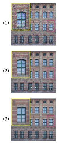
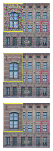
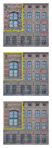
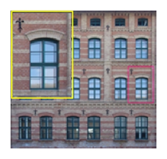
One straightforward application of our algorithm is the image restoration. Same as [12] pointed, our algorithm also assumes the image to be well structured. Though the assumption would not be reasonable for some natural images, it has many applications for visual data such as structured images (e.g., the façade image), CT/MRI data, and multispectral image. In experiments, we apply the algorithm on image restoration of the façade image, which is also used in [12, 17]. We add different percent of random impulsive noise to the image and compare MALM-TR with RSTD. The results produced by both algorithms are shown in Figure 1.

Details are in the caption following the image — **Figure 1 (a)**
Open in figure viewer PowerPoint

Comparisons in terms of visual effects. The rows (1), (2), and (3) correspond to the images before recovery, the obtained results by MALM-TR and RSTD [12], respectively. The columns (a), (b), and (c) correspond to the images corrupted by 15%, 25%, and 35% sparse impulsive noise, respectively. (d) is the original image.

4.3. Background Modeling

Another application of our algorithm is to estimate a good model for the background variations in a scene (i.e., background modeling). In this situation, it is natural to model the background variation as approximately low rank. Foreground objects generally occupy only a fraction of the image pixels and hence can be treated as sparse part.

We test our algorithm using an example from [26] and compare with RSTD [12]. The visual comparisons of the background modeling are shown in Figure 2. It is observed that our algorithm is effective in separating the background which is even a dynamic scene. The results are also comparable to RSTD.

4.4. Traffic Data Recovery

In our previous work [3, 4], we have proposed two tensor-based methods on traffic data application. In [3], a tensor imputation method based on Tucker decomposition is developed to estimate the missing value. As a fact that the exact coordinate and the number of the missing data in the tensor form can be observed and obtained because if an element in the tensor form is missing, it doesn’t have value so we can recognize it easily. While this paper recovers a low-n-rank tensor that is arbitrarily corrupted by a fraction of noise based on the trace norm and ℓ₁-norm optimization. The number and the coordinate of the corrupted data are unknown or not easy to obtain. That means that it is hard to recognize the corrupted data, because the corrupted data have values and hardly be separated from the correct data. The problems solved by the two papers are two different problems. Paper [4] is written from the point of traffic data recovery application which is the same problem that will be solved in this section. The main difference of the two proposed methods is how to use the constraint condition 𝒜 = ℒ + 𝒮. Reference [4] puts the constraint condition to the minimized function with only one parameter γ, which leads the objective function to contain not only tensor but also matrix. However, as the size and structure of each mode of the given tensor data are not always the same, the contribution of each mode of the tensor to the final result may be different. In order to utilize the information of the constraint condition as much as possible, this paper unfolds constraint condition along each mode and use weighted parameters γ_i to obtain the new constraint condition in matrix versions which is put into the minimized function using the augmented Lagrange multiplier strategy. With different objective functions, the optimized process is different too. More details can be found in [4].

In the fourth part of the experiment section, we will apply the proposed algorithm to traffic data recovery. The data used in the experiment are collected by a fixed loop in Sacramento County and downloaded from http://pems.dot.ca.gov/. The period of the data lasts for 77 days from March 14 to May 29, 2011. The traffic volume data are recorded every 5 minutes. Therefore, a daily traffic volume series for a loop detector contains 288 records. To finish traffic data recovery by the proposed algorithm, the first step is to convert the mass traffic data into a tensor form. In this part, we choose 8-week complete traffic volume data from the 77 days. Then, the 8-week data are formed into a tensor model of size 8 × 7 × 288 as Figure 3 shows. In this model, “8” stands for 8 weeks, “7” stands for seven days in one week, and “288” stands for 288 records in one day.

In our previous work [3], the similarity coefficient [27] had been used to analyze the high multimode correlation (“link” mode, “week” mode, “day mode,” and “hour” mode) of traffic data from the point of view of statistic characteristic. For the high multicorrelations of traffic data, the tensor form of size 8 × 7 × 288 can be approximated by a low-n-rank tensor.

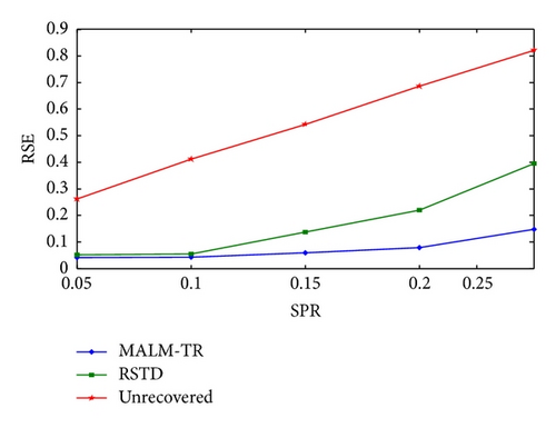
According to the above description, the traffic data are reasonably converted into a tensor form which can be approximated by a low-n-rank tensor. In the traffic data recovery experiment, it is assumed that a subset of entries of the traffic data tensor form is corrupted by impulsive noise at random. The ratios of noisy are set from 5% to 25% with the tolerance 5%. Then we compare the proposed method with RSTD algorithm using RSE as the criterion. The criterion is defined as the following function shows:

()

Table 3 tabulates the RSEs by sparse impulsive noise with different ratio on traffic data. Especially, the unrecovered column presents the RSE between corrupted data and the original data. From data in the table, it is observed that the RSEs obtained by MALM-TR and RSTD are much smaller than the unrecovered data, which means that both algorithm can improve the quality of the corrupted data. Moreover, the RSEs of MALM-TR are smaller than RSTD. From the curves of Figure 4, it is vividly shown that our method performs better than RSTD.

Table 3. Comparison of RSE on traffic data.

SPR	MALM-TR(RSE)	RSTD(RSE)	Unrecovered(RSE)
0.05	0.0406	0.0525	0.2614
0.10	0.0432	0.0543	0.4117
0.15	0.0593	0.1370	0.5427
0.20	0.0784	0.2198	0.6859
0.25	0.1478	0.3959	0.8218

5. Conclusion

In this paper, we extend the matrix recovery problem to low-n-rank tensor recovery and propose an efficient algorithm based on mixture augmented Lagrange multiplier method. The proposed algorithm can automatically separate the low-n-rank tensor data and sparse part. Experiments show that the proposed algorithm is more stable and accurate in most cases and has excellent convergence rate. Different application examples show the broad applicability of our proposed algorithm in computer vision, image processing, and traffic data recovery.

In the future, we would like to investigate how to automatically choose the parameters in our algorithm and develop more efficient method for tensor recovery problem. Also we will explore more applications of our method.

Conflict of Interests

The authors declare that there is no conflict of interests regarding the publication of this paper.

Acknowledgments

The research was supported by NSFC (Grant nos. 61271376, 51308115, and 91120010), the National Basic Research Program of China (973 Program: no. 2012CB725405), and Beijing Natural Science Foundation (4122067). The authors would like to thank Professor Bin Ran from the University of Wisconsin-Madison and Yong Li from the University of Notre Dame for the suggestive discussions.

References

1 Kolda T. G. and Bader B. W., Tensor decompositions and applications, SIAM Review. (2009) 51, no. 3, 455–500, 2-s2.0-68649096448, https://doi.org/10.1137/07070111X.
10.1137/07070111X
Web of Science® Google Scholar
2 Acar E., Dunlavy D. M., Kolda T. G., and Mørup M., Scalable tensor factorizations for incomplete data, Chemometrics and Intelligent Laboratory Systems. (2011) 106, no. 1, 41–56, 2-s2.0-79952446596, https://doi.org/10.1016/j.chemolab.2010.08.004.
10.1016/j.chemolab.2010.08.004
CAS Web of Science® Google Scholar
3 Tan H., Feng G., Feng J., Wang W., Zhang Y. J., and Li F., A tensor-based method for missing traffic data completion, Transportation Research Part C. (2013) 28, 15–27, https://doi.org/10.1016/j.trc.2012.12.007.
10.1016/j.trc.2012.12.007
Web of Science® Google Scholar
4 Tan H., Feng G., Feng J., Wang W., and Zhang Y. J., Traffic volume data outlier recovery via tensor model, Mathematical Problems in Engineering. (2013) 2013, 8, 164810, https://doi.org/10.1155/2013/164810.
10.1155/2013/164810
Web of Science® Google Scholar
5 Vasilescu M. A. O. and Terzopoulos D., Multilinear analysis of image ensembles: Tensorfaces, Proceedings of the European Conference on Computer Vision (ECCV ′02), 2002, 447–460.
Google Scholar
6 Lewis A. S. and Knowles G., Image compression using the 2-D wavelet transform, IEEE Transactions of Image Processing. (1992) 1, no. 2, 244–250, 2-s2.0-0026852760.
10.1109/83.136601
CAS PubMed Web of Science® Google Scholar
7 Sheikh Y. and Shah M., Bayesian modeling of dynamic scenes for object detection, IEEE Transactions on Pattern Analysis and Machine Intelligence. (2005) 27, no. 11, 1778–1792, 2-s2.0-28044439637, https://doi.org/10.1109/TPAMI.2005.213.
10.1109/TPAMI.2005.213
PubMed Web of Science® Google Scholar
8 Itti L., Koch C., and Niebur E., A model of saliency-based visual attention for rapid scene analysis, IEEE Transactions on Pattern Analysis and Machine Intelligence. (1998) 20, no. 11, 1254–1259, 2-s2.0-0032204063, https://doi.org/10.1109/34.730558.
10.1109/34.730558
Web of Science® Google Scholar
9 Chandrasekaran V., Sanghavi S., Parrilo P. A., and Willskyc A. S., Rank-sparsity incoherence for matrix decomposition, http://arxiv.org/abs/0906.2220.
Google Scholar
10 Wright J., Peng Y., Ma Y., Ganesh A., and Rao S., Robust principal component analysis: exact recovery of corrupted low-rank matrices by convex optimization, Proceedings of the 23rd Annual Conference on Neural Information Processing Systems (NIPS ′09), December 2009, 2080–2088, 2-s2.0-84858739923.
Google Scholar
11 Candes E. J., Li X., Ma Y., and Wright J., Robust principal component analysis?, 2009, arXiv:0912.3599v1.
Google Scholar
12 Li Y., Yan J., Zhou Y., and Yang J., Optimum subspace learning and error correction for tensors, Proceedings of the 11th European Conference on Computer Vision (ECCV ′10), 2010, Greece, Crete.
Google Scholar
13 Tucker L. R., Some mathematical notes on three-mode factor analysis, Psychometrika. (1966) 31, no. 3, 279–311, 2-s2.0-0013953617, https://doi.org/10.1007/BF02289464.
10.1007/BF02289464
CAS PubMed Web of Science® Google Scholar
14 Lin Z., Chen M., Wu L., and Ma Y., The augmented Lagrange multiplier method for exact recovery of a corrupted low-rank matrices, Mathematical Programming. (2009) https://doi.org/10.1016/j.jsb.2012.10.010.
10.1016/j.jsb.2012.10.010
Google Scholar
15 Carroll J. D. and Chang J.-J., Analysis of individual differences in multidimensional scaling via an n-way generalization of “Eckart-Young” decomposition, Psychometrika. (1970) 35, no. 3, 283–319, 2-s2.0-34250499792, https://doi.org/10.1007/BF02310791.
10.1007/BF02310791
Web of Science® Google Scholar
16 Harshman R. A., Foundations of the PARAFAC procedure: models and conditions for an “explanatory” multi-modal factor analysis, UCLA Working Papers in Phonetics. (1970) 16, 1–84.
Google Scholar
17 Liu J., Musialski P., Wonka P., and Ye J., Tensor completion for estimating missing values in visual data, Proceedings of the International Conference on Computer Vision (ICCV ′09), 2009.
Google Scholar
18 Liu J., Musialski P., Wonka P., and Ye J., Tensor completion for estimating missing values in visual data, IEEE Transaction on Pattern Analysis and Machine Intelligence. (2013) 35, no. 1, 208–220.
10.1109/TPAMI.2012.39
PubMed Web of Science® Google Scholar
19 Zhou Z., Li X., Wright J., Candès E., and Ma Y., Stable principal component pursuit, Proceedings of the IEEE International Symposium on Information Theory (ISIT ′10), June 2010, 1518–1522, 2-s2.0-77955670622, https://doi.org/10.1109/ISIT.2010.5513535.
10.1109/ISIT.2010.5513535
Google Scholar
20 Bertsekas D. P. and Ozdaglar A. E., Pseudonormality and a lagrange multiplier theory for constrained optimization, Journal of Optimization Theory and Applications. (2002) 114, no. 2, 287–343, 2-s2.0-6344264248, https://doi.org/10.1023/A:1016083601322.
10.1023/A:1016083601322
Web of Science® Google Scholar
21 Bertsekas D., Nonlinear Programming, 1999, Athena Scientific.
Google Scholar
22 Cai J.-F., Candès E. J., and Shen Z., A singular value thresholding algorithm for matrix completion, SIAM Journal on Optimization. (2010) 20, no. 4, 1956–1982, 2-s2.0-77951291046, https://doi.org/10.1137/080738970.
10.1137/080738970
Web of Science® Google Scholar
23 Hale E. T., Yin W., and Zhang Y., Fixed-point continuation for 11-minimization: methodology and convergence, SIAM Journal on Optimization. (2008) 19, no. 3, 1107–1130, 2-s2.0-69649095451, https://doi.org/10.1137/070698920.
10.1137/070698920
Web of Science® Google Scholar
24 Simon H. D., The lanczos algorithm with partial reorthogonalization, Mathematics of Computation. (1984) 42, 115–142, https://doi.org/10.1090/S0025-5718-1984-0725988-X.
10.1090/S0025-5718-1984-0725988-X
Web of Science® Google Scholar
25 Andersson C. A. and Bro R., The N-way toolbox for MATLAB, chemometrics and intelligent laboratory systems, Chemometrics & Intelligent Laboratory Systems. (2000) 52, no. 1, 1–25.4.
10.1016/S0169-7439(00)00071-X
CAS Web of Science® Google Scholar
26 Zhong J. and Sclaroff S., Segmenting foreground objects from a dynamic textured background via a robust Kalman filter, Proceedings of the 9th IEEE International Conference on Computer Vision, October 2003, 44–50, 2-s2.0-0344551957.
Google Scholar
27 Zhang Y. and Liu Y., Missing traffic flow data prediction using least squares support vector machines in urban arterial streets, Proceedings of the IEEE Symposium on Computational Intelligence and Data Mining, CIDM 2009, April 2009, 76–83, 2-s2.0-67650458629, https://doi.org/10.1109/CIDM.2009.4938632.
10.1109/CIDM.2009.4938632
Google Scholar

Citing Literature

All articles

Mixture Augmented Lagrange Multiplier Method for Tensor Recovery and Its Applications

Abstract

1. Introduction

2. Notation and Basics on Tensor Model