Dynamics of an SIR Epidemic Model with Information Variable and Limited Medical Resources Revisited
Abstract
The stability of the SIR epidemic model with information variable and limited medical resources was studied. When the basic reproduction ratio ℛ0 < 1, there exists the disease-free equilibrium and when the basic reproduction ratio ℛ0 > 1, we obtain the sufficient conditions of the existence of the endemic equilibrium. The local asymptotical stability of equilibrium is verified by analyzing the eigenvalues and using the Routh-Hurwitz criterion. We also discuss the global asymptotical stability of the endemic equilibrium by autonomous convergence theorem. A numerical analysis is given to show the effectiveness of the main results.
1. Introduction
Mathematical epidemiology, that is, the building and analysis of mathematical models describing the spread and control of infectious diseases, plays an important role in the areas of biology. Various epidemic models have been proposed and explored extensively and great progress has been achieved in the studies of disease control and prevention. In the classical epidemic models, it is usually assumed that the change of the total population size satisfies logistic model or constant. We used nonlinear incidence, standard incidence rate, general incidence rate, and saturated incidence rate to concentrate on describing the spread of disease through the population. The analysis of all of these models has also been done by some other workers; see for example [1, 2] and the references therein.
In order to control the spread of epidemic, we consider the new variable Z, called information variable which summarizes information about the current state of the disease that is depending on current values of state variables and also summarizes information about past values of state variables. Many authors have used this variable in their models (see, e.g., [3–5]).
In many models, it is usually assumed that the removal rate of the infective is proportional to the number of the infective, which implies that the medical resources such as drugs, vaccines, hospital beds, and isolation places are very sufficient for the infectious disease. However, in reality, every country has an appropriate or limited capacity for treatment. Recently, Kar and Mondal have introduced the continually differentiable treatment function h(I) = rI/(1 + αI) (see in [6]), where r/α models the maximal supply of available medical resources per unit time and 1/(1 + αI) describes the reverse effect of the infected individuals being delayed for treatment, which have important effects on the spread of infectious disease. r/α and the efficiency of the supply of available medical resources 1/(1 + αI) are independent. In many developed countries, in addition to the limitedness of the medical resources, the efficiency of the supply of available medical resources also has an important effect on the transmission of infectious disease, which depends on many factors such as the control strategies and the production of drugs or vaccines. In [7], the SIR models with limited medical resources have been studied.
The paper is organized as follows: in Section 2, we explore the existence of disease-free equilibria point and endemic equilibrium point and investigate the effect of the limited medical resources and their supply efficiency; in Section 3, we analyze the local asymptotic stability of the disease-free equilibria and the endemic equilibrium; in Section 4, we analyze the global asymptotic stability of the endemic equilibrium and present a global analysis of the model; a numerical analysis and a simple discussion are given to conclude this paper in Section 5.
2. The Model and the Existence of Equilibrium
Denote ℛ0 = βk/(μ1 + γ + ε + (b/ω))(1 + kα), .
Theorem 1. (1) The system (6) has a trivial equilibrium E0 = (0,0, 0) and the disease-free equilibrium E1 = (k, 0, k).
(2) If ℛ0 > 1, further if , the system (6) has one endemic equilibrium E* = (S*, I*, Z*) except the disease-free equilibrium.
Proof. (1) Let I = 0, we have S = Z = 0 or S = Z = k; it is not easy to find that the system has a trivial equilibrium and the disease-free equilibrium E0 = (0,0, 0) and E1 = (k, 0, k).
(2) If ℛ0 > 1, from the first question of (6), we have S* = (k/r)(r − (βI*/(1 + αI*))), from the third question of (6), we also have Z* = S*. Then substituting them into the first question of (6) yields
It is clear that if ℛ0 > 1 and , then . We have A < 0, C > 0.
The roots of (7) I1, I2 satisfy
3. The Local Stability Analysis of Equilibria and Bifurcation
In this section, we will examine the local stability of the equilibria by analyzing the eigenvalues of the Jacobian matrices of (6) at the equilibria and using Routh-Hurwitz criterion.
Theorem 2. The free equilibrium point E0 = (0,0, 0) is unstable for any T > 0.
Proof. The Jacobian matrix at E0 is
The eigenvalues are λ1 = r > 0, λ2 = −(μ1 + γ + ε) − (b/ω), and λ3 = −(1/T). Therefore E0 is unstable.
Theorem 3. (1) If ℛ0 > 1, that is, βk > (μ1 + γ + ε + (b/ω))(1 + kα), then E1 = (k, 0, k) is unstable for all T > 0.
(2) If ℛ0 < 1, that is, βk < (μ1 + γ + ε + (b/ω))(1 + kα), then E1 = (k, 0, k) is locally asymptotically stable for all T > 0.
Proof. The Jacobian matrix at E1 is
- (1)
If ℛ0 > 1, that is, (βk/(1 + αk)) > μ1 + γ + ε + (b/ω), then λ2 > 0; therefore E1 = (k, 0, k) is unstable.
- (2)
If ℛ0 < 1, that is, βk/(1 + αk) < μ1 + γ + ε + (b/ω), then λ2 < 0; therefore E1 = (k, 0, k) is locally asymptotically stable.
Note. In Theorem 3, we can see that the stability of disease-free equilibrium point E1 changes from stable to unstable when ℛ0 increases through 1. Therefore, we use ℛ0 as bifurcation parameter.
Theorem 4. The system (6) undergoes transcritical bifurcation at the equilibrium point E0 when bifurcation parameter ℛ0 = 1.
Proof. When ℛ0 = 1, the Jacobian matrix at E1 is
Then J(E1) has a geometrically simple zero eigenvalue with right eigenvector and left eigenvector ψ = (0,1, 0).
Now
According to [9], the system (6) undergoes transcritical bifurcation at the disease-free equilibrium point E1, hence the theorem.
Theorem 5. If ℛ0 > 1 and , then the endemic equilibrium E* is local asymptotical stability for T < T*, where
Proof. The Jacobian matrix at E* is
The characteristic equation is
Let P = (r/k)S*, , and . We have
Let f(T) = (1 + PT)(QT − 1) + (R/(Q − P))T. Then f(0) = −1 and f(T) = 0 has an equine positive root:
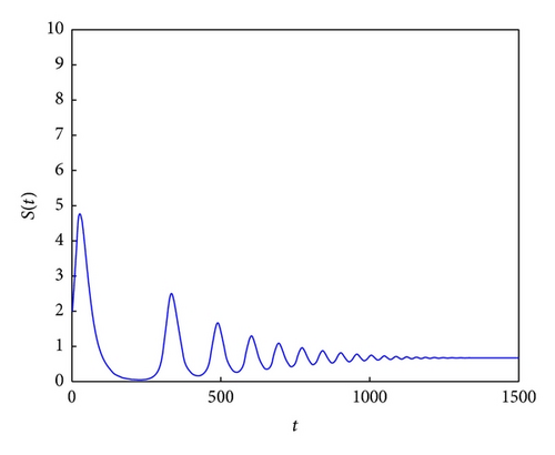
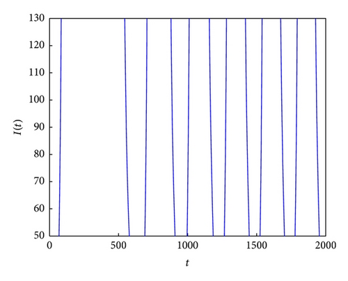
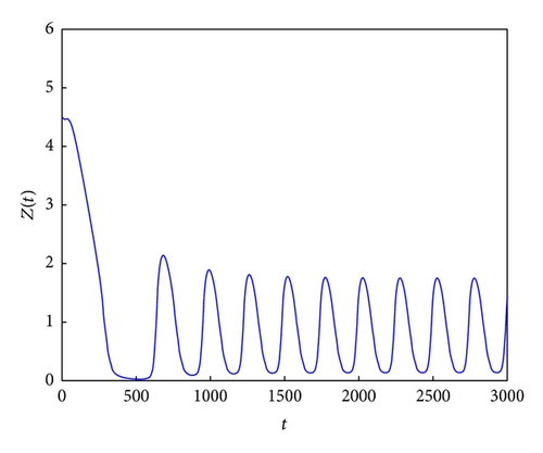
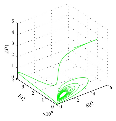
Note. If T > T*, the equilibrium E* may be unstable (see Figure 3).
4. The Global Stability Analysis of the Equilibrium Point
-
(H1) There exists a compact absorbing set K ⊂ D.
-
(H2) Equation (23) has a unique equilibrium x* in D.
The basic idea of this method is that if the equilibrium x* is locally stable, then the stability is assured provided that (H1) and (H2) hold and no nonconstant periodic solution of (23) exists. Therefore, sufficient conditions on f capable of precluding the existence of such solutions have to be detected.
Li and Muldowney showed that if (H1) and (H2) hold and (23) satisfies a Bendixson criterion, that is, robust under C1 local ϵ-perturbations of f at all nonequilibrium nonwandering points for (23), then x* is globally stable robust under C1 local ϵ-perturbation and based on the introduced LozinskiǏ measure.
Lemma 6 (Li and Muldowney [10]). Assume that conditions (H1) and (H2) hold; then x* is globally asymptotically stable in D provided that a function P(x) and a measure μ exist such that (28) is satisfied.
Theorem 7. Under the assumption ℛ0 > 1, , (29), and (30), the endemic equilibrium E* of the system (6) is globally asymptotically stable.
Proof. The Jacobian matrix at E* of system (6) is
Then
Therefore
Consider the norm in R3 as
Therefore
Therefore g1 = (S′/S) − (I′/I) + r − (2rS/k) − (βI/(1 + αI)) + (βI/(1+αZ)2) + (βZ/(1 + αZ)) − (μ1 + γ + ε)−(bω/(ω + I) 2),
From the system (6), I′/I = (βZ/(1 + αZ)) − (μ1 + γ + ε) − (b/(ω + I)); therefore
By integrating both sides at the same time, we obtain
5. Numerical Simulations
- (1)
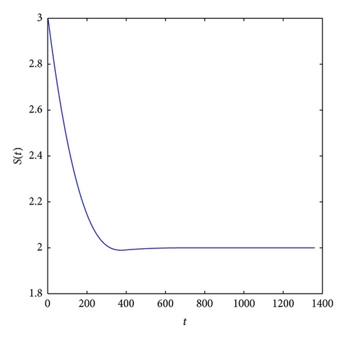
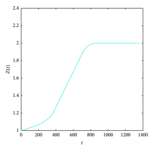
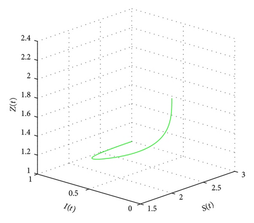
Consider k = 2; β = 0.03; μ1 = 0.1; μ2 = 0.2; r = 3; b = 2; α = 0.001; γ = 0.05; T = 4; ε = 0.02; ω = 12. By directly computing, we obtain R0 = 0.1786 < 1. According to Theorem 3, we know the free disease equilibrium of system (6) is locally asymptotically stable for this case (see Figures 1(a)–1(c) and 1(d)).
- (2)
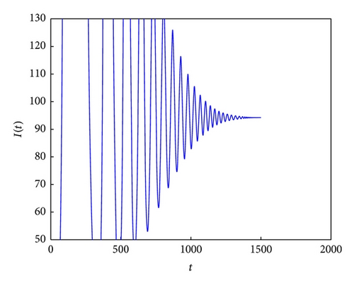
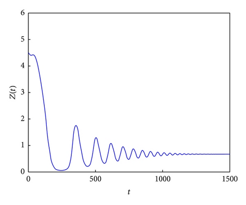
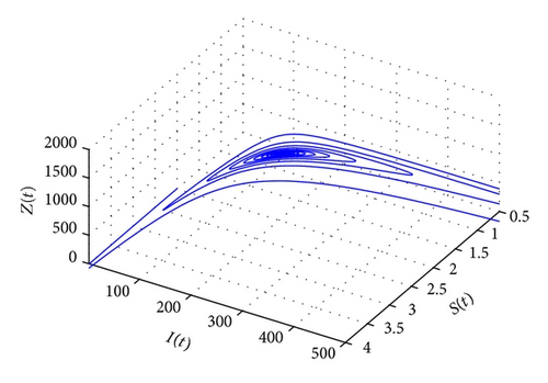
Consider k = 7; β = 0.3; μ1 = 0.1; μ2 = 0.2; r = 3; b = 2; α = 0.1; γ = 0.05; T = 10; ε = 0.02; ω = 12. Through calculation, we know R0 = 3.6692 > 1, T < T*. According to Theorem 7, we know the positive equilibrium of system (6) is locally asymptotically stable for this case (see Figures 2(a)–2(c) and 2(d)).
- (3)
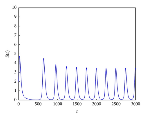
Consider k = 7; β = 0.3; μ1 = 0.1; μ2 = 0.2; r = 3; b = 2; α = 0.1; γ = 0.05; T = 25; ε = 0.02; ω = 12. Through calculation, we know R0 = 3.6692 > 1, T > T*. According to Theorem 5, we know the positive equilibrium of system (6) is unstable for this case (see Figures 3(a)–3(c) and 3(d)).

6. Conclusion
In this paper, the stability of the SIR epidemic model with information variable and limited medical resources has been revisited. By analyzing the model, we have found the disease-free equilibria E0 and E1 exist when the basic reproduction ratio ℛ0 < 1. At the same time we have proved the local asymptotic stability of the disease-free equilibrium. The conclusion reveals that the disease dies out, when ℛ0 > 1; then disease becomes endemic. ℛ0 changes the stability of the disease-free equilibrium and delay parameter T and ω change the stability of the endemic equilibrium. It is shown that the disease-free equilibrium is unstable and the unique endemic equilibrium is globally asymptotically stable under some conditions. Lastly, a numerical simulation provided that, when ℛ0 is less than 1, the disease-free equilibrium is stable and while ℛ0 is more than 1, the disease-free equilibrium is unstable; that is, the endemic equilibrium exists (see Figure 1). We found that if T < T*, the equilibrium E* is globally asymptotically stable (see Figure 2).
If T > T*, it is concluded that the instability of the equilibrium E* has not been studied. It is worthwhile for us to study this case in the future work from the theorematic idea. Here we only illustrate the equilibrium E* is unstable if T > T* by use of the numerical simulation (see Figure 3).
Conflict of Interests
The authors declare that there is no conflict of interests regarding the publication of this paper.
Acknowledgments
The authors would like to thank the anonymous referees for their careful reading of the original paper and their many valuable comments and suggestions that greatly improve the presentation of this work. This work is supported by Natural Science of Shanxi Province (2013011002-2).


