We discuss a new single sweep alternating group explicit iteration method, along with a third-order numerical method based on off-step discretization on a variable mesh to solve the nonlinear ordinary differential equation y^′′ = f(x, y, y^′) subject to given natural boundary conditions. Using the proposed method, we have solved Burgers’ equation both in singular and nonsingular cases, which is the main attraction of our work. The convergence of the proposed method is discussed in detail. We compared the results of the proposed iteration method with the results of the corresponding double sweep alternating group explicit iteration methods to demonstrate computationally the efficiency of the proposed method.

1. Introduction

Consider the general nonlinear ordinary differential equation

()

subject to essential boundary conditions

()

where −∞ < a < b < ∞, A, B are finite constants.

We assume that for x ∈ [a, b], − ∞ < y, z < ∞

(i)
f(x, y, z) is continuous,
(ii)
∂f/∂y and ∂f/∂z exist and are continuous,
(iii)
∂f/∂y > 0 and |∂f/∂z| < W for some positive constant W.

These conditions ensure that the boundary value problem (1) and (2) possesses a unique solution (see Keller [1]).

With the advent of parallel computers, scientists are focusing on developing finite difference methods with the property of parallelism. Working on this, in the early 1980s, Evans [2, 3] introduced the Group Explicit methods for large linear system of equations. Further he discussed the Alternating Group Explicit (AGE) method to solve periodic parabolic equations in a coupled manner. Mohanty and Evans applied AGE method along with various high order methods [4, 5] for the solution of two-point boundary value problems. Later, Sukon and Evans [6] introduced a Two-parameter Alternating Group Explicit (TAGE) method for the two-point boundary value problem with a lower order accuracy scheme. In 2003 Mohanty et al. [7] discussed the application of TAGE method for nonlinear singular two point boundary value problems using a fourth-order difference scheme. In 1990, Evans introduced the Coupled Alternating Group Explicit method [8] and applied it to periodic parabolic equations. Many scientists are applying these parallel algorithms to solve ordinary and partial differential equations [9–11].

Recently, Mohanty [12] has proposed a high order variable mesh method for nonlinear two-point boundary value problem. Mohanty and Khosla [13, 14] also devised a new third-order accurate arithmetic average variable mesh method for the solution of the boundary value problem (1) and (2), using three grid points, which is applicable to both singular and nonsingular problems. No special technique is required to handle singular problems. They also discussed the application of two-parameter double sweep alternating group explicit methods. Here, we discuss a new single sweep group explicit iteration method along with a third-order accurate variable mesh method based on two extra off-step grid points for the solution of the boundary value problem (1) and (2).

2. Off-Step Discretization

Consider the solution interval [a, b] with a nonuniform mesh such that a = x₀ < x₁ < ⋯<x_N < x_N+1 = b. Let h_k = x_k − x_k−1, k = 1(1)N + 1, be the mesh size and let σ_k = h_k+1/h_k > 0, k = 1(1)N, be the mesh ratio. Grid points are given by , i = 1(1)N + 1. Let Y_k = y(x_k) be the exact solution of y at the grid point x_k and approximated by y_k. Let x_k+1/2 = x_k + (σ_kh_k/2) and x_k−1/2 = x_k − (h_k/2).

The new third-order method is described as follows.

For y^′′ = f, we first obtain the off-step discretization

()

where f_k+1/2 = y^′′(x_k+1/2), f_k−1/2 = y^′′(x_k−1/2), and

Now, let

()

Then, at each interior grid point x_k, k = 1(1)N, the proposed differential equation (1) is discretized by

()

With the help of (3), from (5) it is easy to verify that

, provided σ_k ≠ 1. However, for uniform mesh σ_k = 1, the local truncation error associated with (5) becomes

(see Chawla and Shivakumar [15]).

Note that the proposed method (5) is applicable to both singular and nonsingular problems. We do not require any special technique to handle singular problems (see Mohanty [13]). Further note that, the boundary values are given by y₀ = Y₀ = A and y_N+1 = Y_N+1 = B. If the differential equation (1) is linear we use the proposed single sweep AGE iterative method and in nonlinear case, we use the Newton-AGE iterative method to obtain the solution.

3. Application to Singular Problems

3.1. Linear Singular Problems

We now discuss the application of the proposed numerical method (5) to the linear differential equation with variable coefficients

()

where g(x) represents a forcing function.

For D(x) = −α/x and for α = 1 and 2, the equation above represents singular equation in cylindrical and spherical symmetry, respectively.

Let us denote

()

Therefore applying the method (5) to the differential equation (6) and neglecting error term, we obtain a linear difference equation of the form

()

where

()

The linear difference scheme (8) has a local truncation error of and is free from the terms 1/x_k±1 and therefore can very easily be solved for k = 1(1)N in the region x ∈ (0,1).

3.2. Nonlinear Singular Problems

Now we consider the application to nonlinear differential equation (1). Neglecting the error term, we may rewrite the nonlinear difference equation (5) as

()

Let

()

We denote

()

The Jacobian φ(y) may be represented as

()

4. Single Sweep AGE Method

4.1. Description of the Method

In this section we discuss the single sweep AGE iteration method. Using the boundary conditions y₀ = A, y_N+1 = B, the linear difference equation (8) may be written in the matrix form as

()

where

()

To implement the single sweep AGE iterative method, we split the coefficient matrix A into two submatrices A = G₁ + G₂, where G₁ and G₂ satisfy the following conditions.

(i)
G₁ + ω₁I and G₂ + ω₂I are nonsingular for suitable choice of ω₁ > 0 and ω₂ > 0.
(ii)
For any vectors ν₁ and ν₂ and ω₁ > 0, ω₂ > 0, it is “convenient” to solve the system explicitly; that is, and for vectors z₁ and z₂, respectively.

We will be concerned here with the situation where G₁ and G₂ are small (2 × 2) block systems.

Now we discuss the case when N is even (with x₀ = 0, x_N+1 = 1).

Let

()

So that the system (14) can be rewritten as

()

Then a two-parameter AGE method for solving the afore mentioned system may be written as

()

where z^(s) is an intermediate vector.

Eliminating z^(s) and combining (18) and (19), we obtain the iterative method

()

where

()

The new iterative method (20) or (21) is called the two-parameter single sweep AGE iterative method and the matrix T_w is called the iteration matrix.

Now we discuss the single sweep AGE algorithm, when N is even.

For simplicity, we denote

()

and we define d_k = 1/(p_kp_k+1 − c_ka_k+1) for k = 1(1)N − 1.

By carrying out the necessary algebra in (20), we obtain the following algorithm.

For k = 1,

()

For k = 2(2)N − 2.

Let

()

and then

()

Finally, for k = N,

()

Similarly, we can write the single sweep AGE algorithm when N is odd.

4.2. Convergence Analysis

The single sweep AGE iteration method is given by

()

where

()

The matrix T_w is called the iteration matrix.

To prove the convergence of the method, we need to prove that S(T_w) ≤ 1, where S(T_w) denotes the spectral radius of T_w.

Lemma 1. Let h_k be sufficiently small. Then, the eigenvalues of G₁ and G₂ are all real.

Proof. Consider

()

Therefore, we have a_k+1c_k > 0, for k = 1(2)N − 1.

Let λ_i, i = 1(1)N, be the eigenvalues of G₁. Then λ_i’s are the roots of the quadratic equation

()

Simplifying, we get

()

The discriminants of the quadratic equations are

()

Hence, the eigenvalues of G₁ are real.

In a similar manner, we can show that the eigenvalues of G₂ are real.

Now we give the sufficient condition for the convergence of the method.

Theorem 2. Let λ_i and μ_i, i = 1(1)N, be the eigenvalues of G₁ and G₂, respectively. If

()

then the iterative method is convergent for the system (14).

Proof. Let

()

Since the off-diagonal entries of A are negative, therefore a_k+1c_k > 0, k = 1, …, N − 1. Therefore, the diagonal entries of D are positive.

The iteration matrix is given by

()

Define

()

where

and

, and

()

It is easy to verify that

and

are symmetric. Therefore, the matrices

and

are also symmetric. Hence,

()

Also,

is symmetric, and therefore

()

Therefore, we have

()

From (35) and (36), we have ω₁, ω₂ > 0 and λ_i + ω₁ > 0 for k = 1, …, N.

Hence,

()

Also, from (37), we have

()

Hence, we conclude that

()

Thus,

()

Similarly, we can prove that

()

Using (44), (48), and (49), we get S(T_w) < 1.

Hence, the convergence of the method (20) follows.

4.3. Application of Single Sweep Newton-AGE Method

Now we discuss the single sweep Newton-AGE iterative method for the nonlinear difference equation (11). We follow the approaches given by Evans [8, 16].

Let us define

()

Then the Jacobian of φ(y) can be written as the Nth-order tridiagonal matrix

()

Now with any initial vector y⁽⁰⁾, we define

()

where Δy^(s) is the solution of the nonlinear system

()

For the single sweep Newton-AGE method, we consider the case when N is even. We split the matrix T as T = T₁ + T₂, where

()

and then we write single sweep Newton-AGE method as

()

where ω₁ > 0, ω₂ > 0 are relaxation parameters and (T₁ + ω₁I) and (T₂ + ω₂I) are nonsingular.

Since (T₁ + ω₁I) and (T₂ + ω₂I) consist of (2 × 2) submatrices, they can be easily inverted as

()

with p_k = b_k + ω₁, k = 1(1)N, Δ_k = p_kp_k+1 − c_ka_k+1, k = 1(2)N − 1, r_k = b_k + ω₂, k = 1(1)N, and Δ_k = r_kr_k+1 − c_ka_k+1, k = 2(2)N − 2.

The matrices (T₂ + ω₂I) ⁻¹(T₁ + ω₁I) ⁻¹(T₂ − ω₁I) and (T₂ + ω₂I) ⁻¹(T₁ + ω₁I) ⁻¹ can be evaluated in a manner suitable for parallel computing. In order for this method to converge, it is sufficient that the initial vector y⁽⁰⁾ be close to the solution.

Similarly, we can write the single sweep Newton-AGE algorithm when N is odd.

5. Results and Observations

We have applied the methods to the following three examples, whose exact solutions are known to us, and have compared the results with the corresponding double sweep AGE and Newton-AGE method [14]. For single sweep Newton-AGE method, we use the technique given by Evans [16]. The right hand side function and boundary conditions may be obtained using the exact solutions. Here, we have taken σ_k = σ = a constant, k = 1(1)N + 1. The value of the first mesh spacing on the left is given by

()

Therefore, given the value of N and σ, we can calculate h₁ from the above relation and the remaining mesh points are determined by h_k+1 = σh_k, k = 1(1)N. The initial vector y⁽⁰⁾ = 0 is used in all iterative methods and the iterations were stopped when the absolute error tolerance |y^(s+1) − y^(s)| ≤ 10⁻¹⁰ was achieved.

Example 1 (linear singular problem). Consider

()

The exact solution is

. The root mean square errors (RMSE), the maximum absolute errors (MAE), and number of iterations both for single and double sweep AGE methods are tabulated in Table 1 for α = 1, σ = 0.7, α = 2, σ = 1.1, α = 1, σ = 1.0, and α = 2, σ = 1.0. The graph of Example 1 of exact solution versus numerical solution is plotted in Figure 1.

Table 1. Example 1.

N	TAGE			Single sweep AGE			MAE	RMS errors
N	ω₁	ω₂	Iter	ω₁	ω₂	Iter	MAE	RMS errors
α = 1, σ = 0.7
10	0.441	0.44	38	0.47	0.34	20	0.4062 (−03)	0.2435 (−03)
20	0.286	0.286	59	0.33	0.25	33	0.3604 (−03)	0.1558 (−03)
30	0.25	0.247	77	0.32	0.23	44	0.3592 (−03)	0.1269 (−03)
40	0.218	0.218	75	0.24	0.20	47	0.3592 (−03)	0.1099 (−03)
50	0.203	0.203	86	0.26	0.21	54	0.3592 (−03)	0.9829 (−04)
60	0.202	0.199	96	0.26	0.20	62	0.3592 (−03)	0.8973 (−04)
70	0.194	0.194	100	0.26	0.20	65	0.3592 (−03)	0.8307 (−04)
80	0.149	0.149	79	0.25	0.17	62	0.3592 (−03)	0.7771 (−04)

α = 2, σ = 1.1
10	0.529	0.524	39	0.51	0.40	23	0.2990 (−02)	0.2910 (−02)
20	0.298	0.297	78	0.34	0.26	44	0.9774 (−03)	0.9580 (−03)
30	0.213	0.213	113	0.29	0.20	63	0.6774 (−03)	0.6672 (−03)
40	0.169	0.168	146	0.16	0.15	81	0.5925 (−03)	0.5855 (−03)
50	0.142	0.141	178	0.14	0.13	101	0.5633 (−03)	0.5579 (−03)
60	0.124	0.124	180	0.14	0.12	113	0.5525 (−03)	0.5481 (−03)
70	0.112	0.112	201	0.14	0.12	118	0.5484 (−03)	0.5446 (−03)
80	0.103	0.103	221	0.13	0.10	128	0.5469 (−03)	0.5435 (−03)

α = 1, σ = 1.0
10	0.57	0.37	47	0.46	0.34	26	0.4258 (−03)	0.3739 (−03)
20	0.31	0.23	115	0.25	0.239	75	0.3371 (−04)	0.2934 (−04)
30	0.20	0.19	204	0.203	0.183	128	0.7197 (−05)	0.6256 (−05)
40	0.17	0.15	309	0.19	0.17	225	0.2367 (−05)	0.2058 (−05)
50	0.14	0.14	445	0.1749	0.173	362	0.9928 (−06)	0.8634 (−06)
60	0.13	0.13	623	0.179	0.164	503	0.4864 (−06)	0.4232 (−06)
70	0.125	0.124	842	0.177	0.163	681	0.2654 (−06)	0.2310 (−06)
80	0.124	0.123	1117	0.176	0.163	888	0.1567 (−06)	0.1365 (−06)

α = 2, σ = 1.0
10	0.59	0.42	40	0.45	0.39	24	0.5725 (−03)	0.5344 (−03)
20	0.32	0.25	86	0.34	0.25	45	0.4488 (−04)	0.4152 (−04)
30	0.20	0.19	131	0.21	0.18	73	0.9532 (−05)	0.8792 (−05)
40	0.16	0.14	180	0.16	0.14	99	0.3125 (−05)	0.2877 (−05)
50	0.12	0.12	228	0.11	0.10	126	0.1307 (−05)	0.1202 (−05)
60	0.1	0.1	274	0.10	0.09	151	0.6392 (−06)	0.5876 (−06)
70	0.08	0.08	332	0.09	0.08	176	0.3485 (−06)	0.1890 (−06)
80	0.07	0.07	382	0.08	0.07	202	0.2058 (−06)	0.1890 (−06)

Details are in the caption following the image — **Figure 1**
Open in figure viewer PowerPoint

Graph of exact solution and the numerical solution for alpha = 2.0, sigma = 1.1, and N = 80 for Example 1.

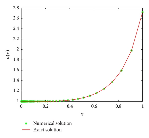
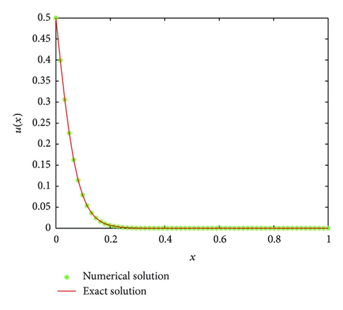
Example 2 (Burgers’ equation). Consider

()

The exact solution is given by y(x) = (1/2)[1 − tanh(x/4v)], where

. The RMSE, MAE, and the number of iterations for both single and double sweep AGE methods are tabulated in Table 2 for R_e = 50, σ = 1.1, R_e = 10, σ = 1.4, and R_e = 50, σ = 1.0. The graph of Example 2 of exact solution versus numerical solution for N = 60, R_e = 50, σ = 1.0 is plotted in Figure 2.

Table 2. Example 2.

N	TAGE			Single sweep AGE			MAE	RMS errors
N	ω₁	ω₂	Iter	ω₁	ω₂	Iter	MAE	RMS errors
R_e = 10, σ = 1.4
10	0.0578	0.0585	6	0.0568	0.0568	6	0.1067(−03)	0.6084(−04)
20	0.0368	0.0374	7	0.0281	0.0285	7	0.8511(−04)	0.3726(−04)
30	0.0318	0.0321	8	0.0320	0.0315	7	0.8442(−04)	0.3028(−04)
40	0.0282	0.0286	9	0.0170	0.0170	8	0.8440(−04)	0.2622(−04)
50	0.0236	0.0239	10	0.0160	0.0166	8	0.8440(−04)	0.2345(−04)
60	0.0161	0.0162	10	0.0161	0.0166	8	0.8440(−04)	0.2141(−04)

R_e = 50, σ = 1.1
10	0.0152	0.0155	5	0.016	0.016	4	0.8156(−03)	0.3181(−03)
20	0.0093	0.0096	6	0.009	0.0089	5	0.3228(−04)	0.1508(−04)
30	0.0063	0.0068	7	0.006	0.0059	7	0.8624(−05)	0.4435(−05)
40	0.0044	0.0045	10	0.0032	0.0042	9	0.5159(−05)	0.2771(−05)
50	0.0036	0.0035	12	0.002	0.0031	12	0.4238(−05)	0.2232(−05)
60	0.0029	0.0029	10	0.0027	0.00278	15	0.3917(−05)	0.1968(−05)

R_e = 50, σ = 1.0
10	0.006	0.014	5	0.005	0.014	4	0.3335(−02)	0.1197(−02)
20	0.012	0.012	5	0.008	0.0089	4	0.3326(−03)	0.9523(−04)
30	0.008	0.008	6	0.008	0.008	4	0.7487(−04)	0.2147(−04)
40	0.0061	0.0061	7	0.0051	0.0053	5	0.2502(−04)	0.7150(−05)
50	0.0049	0.0049	8	0.0058	0.0049	5	0.1055(−04)	0.3012(−05)
60	0.0041	0.0041	9	0.0043	0.0041	5	0.5186(−05)	0.1478(−05)

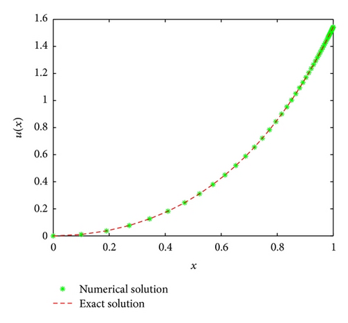
Example 3 (Burgers’ equation in polar coordinates). Consider

()

The exact solution is given by y(x) = x²cosh⁡(x). The RMSE, MAE, and the number of iterations for both single and double sweep AGE methods are tabulated in Table 3 for various values of α, R_e, and σ. The graph of Example 3 of exact solution versus numerical solution for N = 60, R_e = 50, α = 2, σ = 0.9 is plotted in Figure 3.

Table 3. Example 3.

N	TAGE			Single sweep AGE			MAE	RMS errors
N	ω₁	ω₂	Iter	ω₁	ω₂	Iter	MAE	RMS errors
α = 1, R_e = 10, σ = 1.3
10	0.0368	0.0373	8	0.050	0.052	5	0.8036(−03)	0.2692(−03)
20	0.0329	0.0334	9	0.034	0.046	6	0.7645(−03)	0.1770(−03)
30	0.0297	0.0311	10	0.017	0.034	7	0.7605(−03)	0.1436(−03)
40	0.0283	0.0287	10	0.023	0.0242	8	0.7602(−03)	0.1243(−03)
50	0.0261	0.0269	10	0.025	0.027	8	0.7602(−03)	0.1112(−03)
60	0.0242	0.0251	10	0.0211	0.0218	9	0.7602(−03)	0.1015(−03)

α = 2, R_e = 10, σ = 1.2
10	0.0554	0.0562	7	0.0555	0.0559	5	0.6954(−03)	0.2261(−03)
20	0.0457	0.0464	9	0.035	0.037	7	0.4545(−03)	0.1034(−04)
30	0.0403	0.0412	10	0.027	0.029	8	0.4245(−03)	0.7896(−04)
40	0.0381	0.0393	10	0.025	0.030	9	0.4198(−03)	0.6765(−04)
50	0.0359	0.0364	10	0.03	0.033	9	0.4191(−03)	0.6040(−04)
60	0.0326	0.0335	10	0.022	0.029	10	0.4190(−03)	0.5512(−04)

α = 1, R_e = 50, σ = 0.9
10	0.0204	0.0211	8	0.016	0.020	7	0.8035(−03)	0.3961(−03)
20	0.0183	0.0189	8	0.011	0.014	6	0.5906(−03)	0.1492(−03)
30	0.0079	0.0084	9	0.007	0.0072	7	0.5252(−03)	0.1101(−03)
40	0.0056	0.0067	11	0.0051	0.0052	9	0.5044(−03)	0.9227(−04)
50	0.0036	0.0041	15	0.0043	0.0043	12	0.4973(−03)	0.8159(−04)
60	0.0034	0.0035	17	0.0032	0.0034	16	0.4949(−03)	0.7419(−04)

α = 2, R_e = 50, σ = 0.9
10	0.0198	0.0211	8	0.016	0.017	7	0.4542(−03)	0.3755(−03)
20	0.0172	0.0181	8	0.011	0.018	6	0.6976(−04)	0.4929(−04)
30	0.0069	0.0072	9	0.007	0.008	7	0.4018(−04)	0.2422(−04)
40	0.0064	0.0064	10	0.0065	0.0057	8	0.3333(−04)	0.1789(−04)
50	0.0045	0.0043	13	0.0036	0.0041	12	0.3124(−04)	0.1525(−04)
60	0.0035	0.0034	17	0.0043	0.0033	15	0.3054(−04)	0.1372(−04)

α = 1, R_e = 50, σ = 1.0
10	0.0174	0.0177	10	0.01	0.027	8	0.1217(−02)	0.5654(−03)
20	0.009	0.011	12	0.0113	0.0115	9	0.1044(−03)	0.4913(−04)
30	0.0063	0.0065	14	0.0072	0.0077	10	0.4547(−04)	0.1367(−04)
40	0.0063	0.0069	16	0.0054	0.0056	11	0.2617(−04)	0.6119(−05)
50	0.0042	0.0046	18	0.0044	0.0045	12	0.1697(−04)	0.3416(−05)
60	0.0034	0.0039	21	0.0032	0.0041	13	0.1188(−04)	0.2152(−05)

α = 2, R_e = 50, σ = 1.0
10	0.017	0.025	9	0.015	0.026	7	0.1234(−02)	0.5767(−03)
20	0.0101	0.011	11	0.0118	0.0118	9	0.1058(−03)	0.4505(−04)
30	0.0071	0.0083	13	0.0075	0.0075	10	0.2644(−04)	0.1025(−04)
40	0.0054	0.0063	15	0.0049	0.0058	11	0.1502(−04)	0.3813(−05)
50	0.0043	0.0049	17	0.0038	0.0049	12	0.9686(−05)	0.1870(−05)
60	0.0035	0.004	20	0.0042	0.0044	11	0.6762(−05)	0.1084(−05)

6. Discussion and Conclusion

We have discussed a new single sweep AGE iterative method and three-point off-step method of accuracy on a variable mesh for the solution of nonlinear two point boundary value problems. To demonstrate the efficiency of the method, three examples including two nonlinear and singular cases are presented. The results obtained are compared with the corresponding double sweep AGE method and show superiority over the latter. The double sweep AGE method requires two sweeps to solve a problem, whereas the single sweep AGE method requires only one sweep to solve the problem. Experimentally, as compared to the double sweep method the corresponding single sweep method requires much less number of iterations as it uses less intermediate variables. The method can be extended to solve multidimensional problems and is suitable for use on parallel computers.

Conflict of Interests

The authors declare that there is no conflict of interests regarding the publication of this paper.

Acknowledgment

This research was supported by the Council of Scientific and Industrial Research under research Grant no. 09/045(0836)2009-EMR-I.

References

1 Keller H. B., Numerical Methods for Two Point Boundary Value Problems, 1968, Blaisdell.
Google Scholar
2 Evans D. J., Parallel strategies for linear systems of equations, International Journal of Computer Mathematics. (2004) 81, no. 4, 417–446, 2-s2.0-28244478399, https://doi.org/10.1080/00207160310001606061.
Google Scholar
3 Evans D. J., Group explicit methods for solving large linear systems, International Journal of Computer Mathematics. (1985) 17, 81–108.
Google Scholar
4 Evans D. J. and Mohanty R. K., Alternating group explicit method for the numerical solution of non-linear singular two-point boundary value problems using a fourth order finite difference method, International Journal of Computer Mathematics. (2002) 79, no. 10, 1121–1133, 2-s2.0-4944257588, https://doi.org/10.1080/00207160212704.
Google Scholar
5 Mohanty R. K. and Evans D. J., A fourth order accurate cubic spline alternating group explicit method for non-linear singular two point boundary value problems, International Journal of Computer Mathematics. (2003) 80, no. 4, 479–492, 2-s2.0-28244464374, https://doi.org/10.1080/0020716021000009219.
Web of Science® Google Scholar
6 Sukon K. S. and Evans D. J., Two parameter AGE (TAGE) method for the solution of a tri-diagonal linear system of equations, International Journal of Computer Mathematics. (1996) 60, no. 3-4, 265–278, 2-s2.0-0029698441.
Google Scholar
7 Mohanty R. K., Sachdev P. L., and Jha N., TAGE Method for nonlinear singular two point boundary value problems using a fourth order difference scheme, Neural, Parallel and Scientific Computations. (2003) 11, 281–287.
Google Scholar
8 Evans D. J., The solution of periodic parabolic equations by the coupled alternating group explicit (CAGE) iterative method, International Journal of Computer Mathematics. (1990) 34, 227–235.
Google Scholar
9 Evans D. J. and Pragya Jain, The coupled reduced alternating group explicit (CRAGE) method, Parallel Algorithms and Applications. (1993) 2, 193–208.
Google Scholar
10 Feng Q., Explicit finite difference method for convection-diffusion equations, 2, Proceedings of the World Congress on Engineering, 2009, London, UK, 1094–1097.
Google Scholar
11 Zheng B. and Feng Q., Parallel finite difference method for diffusion equations, Proceedings of the 15th American Conference on Applied Mathematics, 2009, 60–62.
Google Scholar
12 Mohanty R. K., A family of variable mesh methods for the estimates of (du/dr) and solution of non-linear two point boundary value problems with singularity, Journal of Computational and Applied Mathematics. (2005) 182, no. 1, 173–187, 2-s2.0-19644383361, https://doi.org/10.1016/j.cam.2004.11.045.
Google Scholar
13 Mohanty R. K., A class of non-uniform mesh three point arithmetic average discretization for y^″ = f(x, y, y^′) and the estimates of y^′, Applied Mathematics and Computation. (2006) 183, no. 1, 477–485, 2-s2.0-33845434623, https://doi.org/10.1016/j.amc.2006.05.071.
Google Scholar
14 Mohanty R. K. and Khosla N., Application of TAGE iterative algorithms to an efficient third order arithmetic average variable mesh discretization for two-point non-linear boundary value problems, Applied Mathematics and Computation. (2006) 172, no. 1, 148–162, 2-s2.0-31144452443, https://doi.org/10.1016/j.amc.2005.01.134.
Google Scholar
15 Chawla M. M. and Shivakumar P. N., An efficient finite difference method for two-point boundary value problems, Neural, Parallel & Scientific Computations. (1996) 4, no. 3, 387–395, MR1418131, ZBL1060.65626.
Google Scholar
16 Evans D. J., Iterative methods for solving non-linear two point boundary value problems, International Journal of Computer Mathematics. (1999) 72, no. 3, 395–401, 2-s2.0-0345912811.
Google Scholar

All articles

A Single Sweep AGE Algorithm on a Variable Mesh Based on Off-Step Discretization for the Solution of Nonlinear Burgers’ Equation

Abstract

1. Introduction

2. Off-Step Discretization