Volume 2014, Issue 1 731272

Research Article

Open Access

A Fast Alternating Minimization Algorithm for Nonlocal Vectorial Total Variational Multichannel Image Denoising

Corresponding Author

Rubing Xi

[email protected]

Department of Mathematics and Systems Science, National University of Defense Technology, Changsha 410073, China nudt.edu.cn

Search for more papers by this author

Zhengming Wang,

Zhengming Wang

Department of Mathematics and Systems Science, National University of Defense Technology, Changsha 410073, China nudt.edu.cn

Search for more papers by this author

Xia Zhao,

Xia Zhao

Department of Mathematics and Systems Science, National University of Defense Technology, Changsha 410073, China nudt.edu.cn

Search for more papers by this author

Meihua Xie,

Meihua Xie

Department of Mathematics and Systems Science, National University of Defense Technology, Changsha 410073, China nudt.edu.cn

Search for more papers by this author

Rubing Xi,

Corresponding Author

Rubing Xi

[email protected]

Department of Mathematics and Systems Science, National University of Defense Technology, Changsha 410073, China nudt.edu.cn

Search for more papers by this author

Zhengming Wang,

Zhengming Wang

Department of Mathematics and Systems Science, National University of Defense Technology, Changsha 410073, China nudt.edu.cn

Search for more papers by this author

Xia Zhao,

Xia Zhao

Department of Mathematics and Systems Science, National University of Defense Technology, Changsha 410073, China nudt.edu.cn

Search for more papers by this author

Meihua Xie,

Meihua Xie

Department of Mathematics and Systems Science, National University of Defense Technology, Changsha 410073, China nudt.edu.cn

Search for more papers by this author

First published: 26 August 2014

https://doi.org/10.1155/2014/731272

Citations: 1

Academic Editor: Zhike Peng

Share a link

Email
Wechat
Bluesky

Abstract

The variational models with nonlocal regularization offer superior image restoration quality over traditional method. But the processing speed remains a bottleneck due to the calculation quantity brought by the recent iterative algorithms. In this paper, a fast algorithm is proposed to restore the multichannel image in the presence of additive Gaussian noise by minimizing an energy function consisting of an -norm fidelity term and a nonlocal vectorial total variational regularization term. This algorithm is based on the variable splitting and penalty techniques in optimization. Following our previous work on the proof of the existence and the uniqueness of the solution of the model, we establish and prove the convergence properties of this algorithm, which are the finite convergence for some variables and the q-linear convergence for the rest. Experiments show that this model has a fabulous texture-preserving property in restoring color images. Both the theoretical derivation of the computation complexity analysis and the experimental results show that the proposed algorithm performs favorably in comparison to the widely used fixed point algorithm.

1. Introduction

The restoration of multichannel image is one of the most important inverse problems in image processing. Among all the methods for restoration, the vectorial total variational (VTV) regularization is most popular for preserving discontinuities in restored images. VTV has been introduced by [1] into multichannel image restoration as a vectorial extension of total variation (TV) in gray scale image processing.

The famous total variational (TV) methods have drawbacks due to its local property while calculating the gradient of the image. Thus the images that contain many small structures or textures cannot get satisfying restored results. As a result, TV method based on nonlocal (NL) operator is generally used in gray scale image processing because of its structure preserving property. This method is generalized from the Yaroslavsky denoising and the block method. The main idea is using the similar blocks in the whole image to estimate current pixel value. It was introduced by Efros and Leung [2] while studying texture synthesis. Then Buades et al. [3] generalized nonlocal method and proposed the well-known neighbor denoising filter, namely, nonlocal means (NLM). After that, Gilboa and Osher [4] united nonlocal method into the regularization framework by defining the nonlocal formed TV model including NL-TV- model, NL-TV- model, and NL-TV-G model and proposed the algorithms separately. NL-TV model can both preserve the edges and the other small structures in images and has excellent application effect.

Our previews works extends NL-TV regularization to NL-VTV regularization for multichannel image restoration (see [5]). The corresponding algorithms are based on the variation calculus by solving the Euler-Lagrangian equations by fixed point iterations. This kind of methods is tested effectively but has a low convergence rate.

Recently, the optimization algorithms based on variable-splitting and penalty techniques have attracted much attention in image and signal processing, such as the dual methods, the Bregman methods, and the alternating direction method of multipliers (ADMM) methods (see [6–8]). Correspondingly, these methods have been extended for multichannel images. Bresson and Chan [6] has extended Chambolle’s dual algorithm for TV problem to vectorial images by defining the standard dual definition of VTV. Wang et al. [9, 10] has applied the alternating minimization algorithm to VTV model for multichannel image deblurring.

In this paper, we propose a fast alternating algorithm for NL-VTV model to restore color images from noisy observations. The following sections are organized as follows. Section 2 is the brief introduction of the NL-VTV model and classical fixed point algorithm. In Section 3, we propose the alternating algorithm for NL-VTV model. In Section 4, we do the convergence analysis of this algorithm. In Section 5, we applied this algorithm to color image denoising to present the texture-preserving effect of the NL-VTV model and the high convergent rate of the proposed algorithm.

2. Nonlocal Vectorial Total Variation Model

In this section, we will briefly introduce the nonlocal vectorial total variational model for multichannel image processing. The usually used iterative algorithm will be introduced as well, which will be compared to our algorithm in Section 5.

2.1. Vectorial Total Variation Model

Consider a vector valued function u, such as the multichannel images, defined on a bounded open domain

(1)

where

denotes the mth channel of u.

The regularized VTV model for multichannel image reconstruction could be written as

(2)

where u₀ is the observed noisy multichannel image and λ > 0 is the regularized parameter. The vectorial gradient of u is defined as

(3)

We refer to [6] for more information about the well-posedness analysis of the VTV model.

2.2. Nonlocal Functional

The neighborhood filter NLM proposed by Buades et al. developed to a famous image denoising method [3]. It uses the pixels similar to the current pixel to estimate the value of the current pixel. Let the reference image be ν. The similarity of the two pixels in the image x, y could be measured as the following weight function w_ν(x, y):

(4)

where G_a is the Gaussian kernel with the standard deviation of a:

(5)

where h is the filter parameter. Generally, h corresponds to the noise level, which is usually set as the standard deviation of the noise. It is shown that the weight function above could be calculated by the image blocks centered around x, y. The value of the weight function reflects the similarity of the two blocks. The estimation of the value at pixel x by the nonlocal means is

(6)

where the normalized factor C(x) = ∫_Ωw_ν(x, y)dy. It can be seen that this method is a kind of special filter algorithm, and the estimation of the value at pixel x is weighted by the values of all the pixels y (y ∈ Ω) in the image.

Let the 2-dimensional image domain be

, pixels x ∈ Ω, and u(x) is a real function on

. The derivation under the nonlocal frame is

(7)

where

is the nonnegative symmetrical weight function defined as (4), which is calculated by the reference image.

The nonlocal gradient ∇_wu(x, y) is defined as a vector composed by all the partial derivations at position x: ∇_wu(x, ·), where ∇_wu : Ω → Ω × Ω:

(8)

Define the nonlocal divergence as

(9)

which satisfies the conjugation with the nonlocal gradient; that is,

(10)

Thus the nonlocal Laplacian is defined as

(11)

The NL-TV norm of u ∈ L¹(Ω) based on nonlocal operators, that is, the weighted gradient ∇_wu, is defined by

(12)

where function w(x, y) is defined as (4). The NL-TV model can be written as

(13)

The well-posedness of NL-TV model is guaranteed in [11].

2.3. Nonlocal Vectorial Total Variation Model and the Fixed Point Iterative Algorithm

In this section, the nonlocal gradient will be introduced to reconstruct the variation norm in the vectorial total variation model to deduce the NL-VTV model.

The vectorial nonlocal gradient could be derived by generalizing the nonlocal gradient defined previously:

(14)

where

, m = 1, …, M, represents the gradient of each channel separately, which is calculated by the image of its own channel.

Use the vectorial nonlocal gradient ∇_wu to replace the gradient ∇u in VTV norm; we get the NL-VTV model:

(15)

where ∫_Ω | ∇_wu | dx is the VTV regularization based on the nonlocal gradient, which could be denoted by

(16)

The existence and the uniqueness of the solution to (15) have been proven in our previews work, in which we proposed a fixed point iterative algorithm to solve (15) as well. Here we will give out a brief introduction as follows.

The Euler-Lagrangian equation of the functional (15) is

(17)

Calculate the nonlocal curvature channel by channel; that is,

(18)

where

, m = 1, …, M. Then the Euler-Lagrange equation becomes

(19)

According to (19), when the weight function is fixed, the Euler-Lagrange equation is linear, which could be solved by the gradient descent kind of algorithm as follows.

First of all, we discretize (19). Denote

to be the pixel value at position i of the mth channel image, where 1 ≤ m ≤ M, 1 ≤ i ≤ N (if the size of the image is a × b, N = a × b).

is the discrete value of the weight function w(x, y), that is, the weight function value with respect to pixel i and pixel j. The pixel j traverses the image channel where the pixel i is in. Denote the neighbor set to be

, where τ denotes a threshold value as a judgment of the similarity between the two blocks centered at pixel i and pixel j, respectively. Let ∇_wd be the discrete ∇_w:

(20)

And let div_wd be the discrete div_w:

As for functions, the discrete inner product is 〈u, v〉≔∑_i(u_iv_i), while, as for vectors, the discrete dot product is (p, q) _i≔∑_j(p_i,jq_i,j), the discrete inner product is 〈p, q〉≔∑_i∑_j(p_i,jq_i,j). The norm of vector is .

Then for channel m, where 1 ≤ m ≤ M, the discrete nonlocal curvature is

(21)

where

and

. Then the Euler-Lagrange equation becomes

(22)

Denote

. Then the Euler-Lagrange equation could be shortly written as

(23)

Furthermore, it could be written as

(24)

According to the fixed point iteration, we use the multichannel image u(k) in step k to update image u(k + 1) in step k + 1. The weights are calculated by the original observation image. Then we get the iteration formula as

(25)

where i ∈ Ω,

The convergence property of the fixed point algorithm has been proved in our in-press work. However, when |∇_wu | = 0, the NLTV functional is nondifferentiable, which is similar to the classical TV model. Thus a regularization is involved in the calculation of to escape the denominator to be zero. Consequently, this algorithm takes many iteration steps to obtain the best restoration result. Thus we consider designing a fast alternating minimization algorithm instead.

3. The Alternating Minimization Algorithm

For the sake of conquering the nondifferentiability of the VTV functional, we design an alternating minimization algorithm in this section to solve the problem (15). The main idea of the alternating minimization is introducing an auxiliary variable. Then the original problem could be split into two subproblems of which one is differential with respect to the original variable, while the other is convex with respect to the auxiliary variable, respectively.

Yang et al. [10] have already studied the alternating minimization algorithm for a general model:

(26)

Model (26) reduces to (15) when G_i = I_m ⊗ ∇_w, α_i = 1, and K = I, where I_m is the identity matrix of order m and ⊗ represents the Kronecker product. Yang et al. pointed out in [10] that if G_i is the finite difference operator D_i, then, under some boundary conditions for u and some other assumptions for the blurring kernel K, the problem (26) can be fast transformed by fast Fourier transform, which diagonalizes the block circulant matrices: D_i, K, and their transpose, and then can be solved by the fast algorithm such as the Gaussian elimination method.

However, the nonlocal gradient operator ∇_w in (15) is not block circulant. We will figure out another method to speed up the algorithm. We briefly propose the algorithm in this section. The convergence of this algorithm will be analysed in Section 4, as well as others properties of this algorithm.

3.1. Variable Splitting (Half-Quadratic Formulation of (15))

We introduce an auxiliary variable d to approximate the nonlocal gradient of u, that is, ∇_wu. Then the minimization problem (15) is transformed into an equivalent constrained problem:

(27)

In order to solve problem (27), we use the penalty method to reformulate it as

(28)

where β is the penalty parameter. It could be easily proved that, as β → ∞, the solution of problem (28) is convergent to the solution of problem (15).

3.2. Alternating Minimization Algorithm

The problem of minimizing (28) with respect to d for fixed u becomes

(29)

The functional in (29) is convex with respect to d. According to Lemma 3.3 in [10], the problem (29) has the unique solutions given by

(30)

where the multidimensional shrinkage operator shrink(x, λ) = (x/|x|) · max⁡{|x | − λ, 0}.

On the other hand, minimizing (28) with respect to u for fixed d becomes

(31)

The functional in (31) is differential with respect to u. Thus the solution to (31) satisfies the first order optimized condition; that is, the Euler-Lagrange equation of the functional (31) is

(32)

After some steps of simple calculation, we get

(33)

Then according to (11), we get

(34)

Finally, the multichannel image u is calculated as follows:

(35)

Since the graph Laplacian Δ_w is negative semidefinite, the operator I − (2β/λ)Δ_w is diagonally dominant. Therefore we can solve u^k+1 by a Gauss-Seidel algorithm. However, the subproblem (35) consists in solving the linear equations with the scale of N × N for each image channel. As a result, the calculation complexity of the Gauss-Seidel algorithm is heavy. We are inspired by Chen and Cheng [12] to simplify, and, without loss of generality as well, we chose λ = β². Furthermore, using Taylor expansion to approximate, there is

(36)

where

is the weight matrix of similar blocks of each channel, which is normalized to a symmetrical matrix with the sum of every row equal to 1. Thus the solution to (35) is

(37)

According to (9), the divergence at pixel i is

, m = 1, …, M.

To conclude this section, we rewrite the alternating minimization algorithm as in Table 1.

Table 1. Comparison of the highest SNR obtained.

SNR	Noisy image	VTV	NLVTV
Barbara image	8.9013	13.1212	13.2873
Baboon image	9.2373	13.1618	12.5936

4. Convergence Analysis

Since it has been proved in our in-press work that the model (15) has the unique solution, in this section, we prove that the solution obtained by Algorithm 1 is the unique one. First, the convergence of the quadratic penalty method as the penalty parameter goes to infinity is well known [13]. That is, as β → ∞, the solution of (31) converges to that of (15). We analyze the convergence properties of Algorithm 1 for a fixed β > 0. In this section, we show that, for any fixed β, the algorithm of minimizing u and d alternately has finite convergence for some variables and q-linear convergence for the rest.

Algorithm 1: Alternating minimization algorithm for nonlocal VTV denoising.

Initialization:
for k = 0 to K, do
Solve d^k+1 = shrink(∇_wu^k+1, 1/β).
Solve u^k+1 = (1 − (2/β))I(u₀ − (1/β)div_wd^k)+(2/β)W(u₀ − (1/β)div_wd^k).
end for

Theorem 1. The iterative sequence {(d^k, u^k)} generated by (30) and (37) from any starting point {(d⁰, u⁰)} converges to the solution of the minimization problem (31).

Proof. According to (30) and (37), the functional E(u, d) in (28) satisfies

(38)

Therefore, the sequence {E(u^k, d^k)} is nonincreasing. Thus it is convergent in because of its nonnegativity as well. We denote the limit of the sequence by m. We prove that m = E(u^*, d^*) followed, where u^* and d^* are the solution of (31).

Because E is coercive and the sequence {E(u^k, d^k)} is convergent, the sequence {(u^k, d^k)} is bounded. Thus there exists a subsequence {(u^k, d^k)}, which converges to an accumulation point when n_k → ∞. According to (30) and (37), for all , d,

(39)

and, for all

, u,

(40)

We denote as the accumulation point of the sequence , because of that the functional E is continuous, according to (38),

(41)

Because of that the threshold function, shrink, in (30), is continuous, we compute the limits of both sides of the equation and get

(42)

Thus . According to (41), . On the other hand, E is strictly convex with respect to d, then we have because of the uniqueness of the minimizer of . Similarly, we prove that .

We compute the limits of (39) and (40),

(43)

According to (43), . Thus the limit points of all of the subsequence of {(u^k, d^k)} are the solutions to (28). As a result, {(u^k, d^k)} converges to (u^*, d^*).

Let S_1/β(∇_wu) = shrink(∇_wu, 1/β) and let P = (I − (2β/λ)Δ_w) ⁻¹. We define set , where ν < 1 is a positive constant. Then we have the following conclusion.

Theorem 2 (q-linear convergence). Assume that the sequence ; then there is a constant β₀ > 0, such that for all β > β₀, the sequence {u^k} generated by (30) and (37) is q-linear convergence.

Proof. Combine (30) and (37); we have

(44)

We know that u^* is a fixed point of (44). Let Q = P⁻¹ = I − (2β/λ)Δ_w = (1 + (2/β))I − (2/β)W. Then

(45)

Since the operator S_1/β is nonexpansive,

(46)

Because

(47)

We write τ = 1/(1 + (2/β)−(2/β)ν) < 1. Then by uniting (46) and (47), we have

(48)

Let . Then for all β > β₀, the sequence {u^k} generated by (30) and (37) is q-linear convergent to u^*.

5. Experiments

In this section, we apply Algorithm 1 to color image denoising to test its efficiency. We compare this method to that in [10] to show the detail-preserving property of the nonlocal VTV model. Then we compare the convergent rate of this algorithm with the fixed point algorithm presented in Section 2.

5.1. Texture-Preserving Property of the NLVTV Model

We choose the color Barbara picture size 300 × 300 × 3 and the color Baboon picture size 256 × 256 × 3 for testing, both of which contain many textures, such as the woman’s scarf and the baboon’s beard. We add the Gaussian white noise with standard deviation 20 to the two original pictures. Then we use the VTV model and the NLVTV model to restore them, separately. In this experiment, the signal to noise rate (SNR) is used to estimate the restoration effect of the methods, which is defined as follows:

(49)

where var(x) represents the variance of all the elements of matrix x.

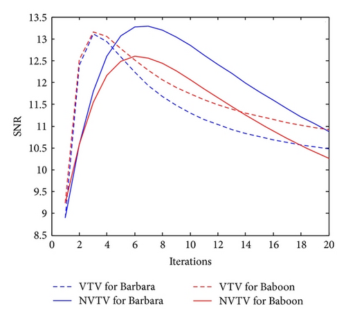
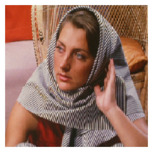
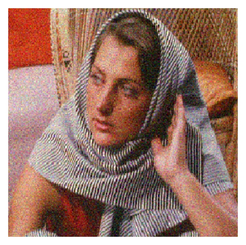
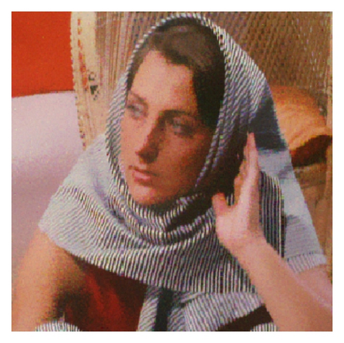
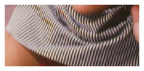
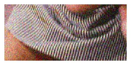
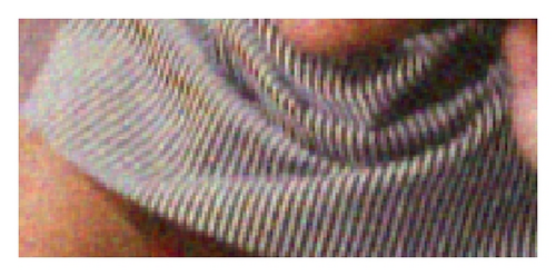
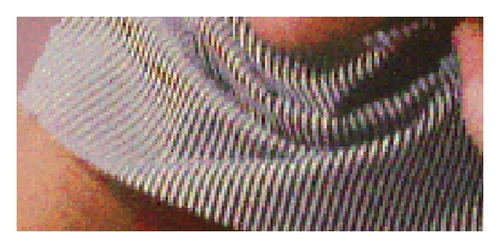
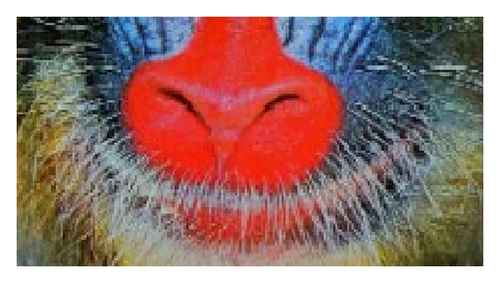
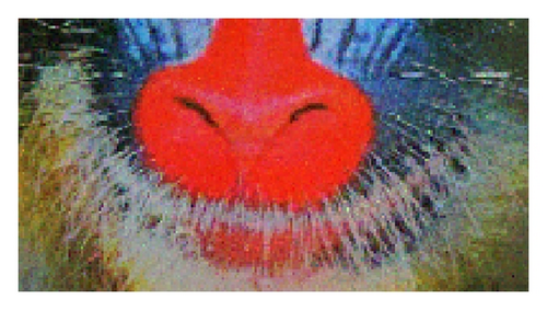
As is shown in Figure 1 and Table 1, the NLVTV model obtains similar SNR to VTV model. In the experiment of restoring the color Barbara picture, we choose the restored image by NLVTV model under the SNR (13.0678) lower than but close to that of the VTV model (SNR = 13.1212) instead of the restored image under the best SNR (13.2873). Figure 2 shows the results. Figure 3 shows the zoom part of the restored image, that is, the woman’s scarf. We can see that the NVTV model preserves the details better than the VTV model. Figures 4 and 5 show the results of the experiment of restoring the color Baboon picture. Although the NLVTV model gets lower SNR than the VTV model, the textures in this picture are better preserved by the NLVTV model rather than the VTV model.

Details are in the caption following the image — **Figure 1**
Open in figure viewer PowerPoint

Comparison of SNR.

5.2. Computation Complexity Analysis and the Convergent Rate Comparison

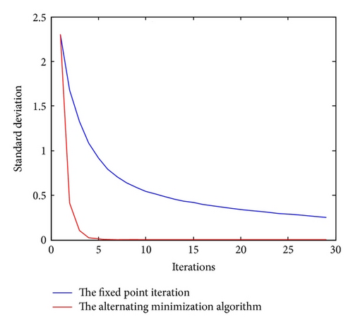
In this section, we compare the computation complexity and the convergent rate of this algorithm to the fixed point algorithm.

First, we analyze the computation complexities of the two algorithms, respectively. Assume the size of the multichannel image is n × n × M. The size of the nonlocal searching window is m × m. We do not consider the computation complexity of the calculation of the nonlocal weight, because that is executed exactly the same in both algorithms.

At each iterative step of Algorithm 1, namely, (30) and (37), the dominant calculation of (30) contains the calculation of the nonlocal gradient and the threshold computation of M(nm) ² times. Thus the computation complexity is O(Mn⁴) + O(M(nm) ²). The dominant calculation of (37) contains a step of nonlocal divergence computation with the computation complexity of O(Mn²) and a matrix multiplication with the computation complexity of O(Mn⁴). As a result, the total computation complexity for each iteration is O(Mn⁴) + O(M(nm) ²) + O(Mn²) + O(Mn⁴).

On the other hand, each iterative step of the fixed point iteration contains the nonlocal curvature with the computation complexity of O(Mn⁴) and three matrix multiplications with the computation complexity of O(Mn⁴) + O(Mn⁴) + O(Mn⁴). As a result, the total computation complexity for each iteration is O(Mn⁴) + O(Mn⁴) + O(Mn⁴) + O(Mn⁴).

Consequently, the computation complexity of the proposed algorithm is much less than the fixed point algorithm.

The convergence rate can be represented by the relationship between the iterative step and the standard deviation of the restored image, intuitively. Figure 6 shows the comparison of the convergence rate between the fixed point iteration and the proposed alternating minimization algorithm. The horizontal axis represents the iterative step. And the vertical axis represents the standard deviation of the restored image in each step. The standard deviation is calculated as

(50)

where u^k and u^k−1 represent the restored images of step k and step k − 1, respectively. When calculating std(x), we reshape matrix x into a vector x whose elements are taken column-wise from matrix x. Then

(51)

Figure 6 shows that the alternating minimization algorithm converges faster.

6. Conclusion

In this paper, we propose a fast alternating minimization algorithm for multichannel image processing, based on the new nonlocal vectorial total variational model introduced recently. We use the variable splitting and penalty techniques to split the energy minimization problem into two optimization subproblems. One is a simple minimization problem, which is solved by the threshold method. The other is a simple minimization problem, which is solved by the variation calculus. As a result, this algorithm is faster than the classical algorithm because of avoiding dealing with the nondifferentiability of the nonlocal TV norm.

The main contribution of this paper is introducing the alternating minimization algorithm for the nonlocal vectorial total variational model, which is proved fast and can be applied to many multichannel image processing problems. In this paper, we apply this algorithm to the RGB color image denoising as an example. It can be easily extended to other vectorial problems, such as color image deblurring, and to other color image models, such as hue-saturation-value (HSV) model, as well.

Conflict of Interests

The authors declare that there is no conflict of interests regarding the publication of this paper.

Acknowledgments

This paper and the related works are supported by grants from the National Natural Science Foundation of China under Contracts 61072142, 61271437, and 61201337 and the Science Research Project of National University of Defense Technology under Contracts JC12-02-05 and JC13-02-03.

References

1 Sapiro G. and Ringach D. L., Anisotropic diffusion of multivalued images with applications to color filtering, IEEE Transactions on Image Processing. (1996) 5, no. 11, 1582–1586, https://doi.org/10.1109/83.541429, 2-s2.0-0030286977.
10.1109/83.541429
CAS PubMed Web of Science® Google Scholar
2 Efros A. A. and Leung T. K., Texture synthesis by non-parametric sampling, Proceedings of the 7th IEEE International Conference on Computer Vision (ICCV ′99), September 1999, Kerkyra, Greece, 1033–1038, 2-s2.0-0033285309.
Google Scholar
3 Buades A., Coll B., and Morel J. M., A review of image denoising algorithms, with a new one, Multiscale Modeling & Simulation. (2005) 4, no. 2, 490–530, https://doi.org/10.1137/040616024, MR2162865, 2-s2.0-33645653318.
10.1137/040616024
Web of Science® Google Scholar
4 Gilboa G. and Osher S., Nonlocal operators with applications to image processing, cam report, 2007, no. 07-23, UCLA.
Google Scholar
5 Xi R., Wang Z., and Zhao X., A non-local means based vectorial total variational model for multi-channel SAR image denoising, Proceedings of the 6th International Congress on Image and Signal Processing (CISP ′13), 2013, 217–222.
Google Scholar
6 Bresson X. and Chan T. F., Fast dual minimization of the vectorial total variation norm and applications to color image processing, Inverse Problems and Imaging. (2008) 2, no. 4, 455–484, https://doi.org/10.3934/ipi.2008.2.455, MR2558277, ZBL1188.68337.
10.3934/ipi.2008.2.455
Web of Science® Google Scholar
7 Yin W., Osher S., and Goldfarb D., Bregman iterative algorithms for ℓ1-minimization with applications to compressed sensing, SIAM Journal on Imaging Sciences. (2008) 1, no. 1, 143–168, https://doi.org/10.1137/070703983.
10.1137/070703983
Web of Science® Google Scholar
8 Boley D., Local linear convergence of the alternating direction method of multipliers on quadratic or linear programs, SIAM Journal on Optimization. (2013) 23, no. 4, 2183–2207, https://doi.org/10.1137/120878951, MR3123832, ZBL1288.65086.
10.1137/120878951
Web of Science® Google Scholar
9 Wang Y., Yang J., Yin W., and Zhang Y., A new alternating minimization algorithm for total variation image reconstruction, SIAM Journal on Imaging Sciences. (2008) 1, no. 3, 248–272, https://doi.org/10.1137/080724265, MR2486032, ZBL1187.68665.
10.1137/080724265
Web of Science® Google Scholar
10 Yang J., Yin W., Zhang Y., and Wang Y., A fast algorithm for edge-preserving variational multichannel image restoration, SIAM Journal on Imaging Sciences. (2009) 2, no. 2, 569–592, https://doi.org/10.1137/080730421, MR2519923, ZBL1181.68304.
10.1137/080730421
Web of Science® Google Scholar
11 Bresson X. and Chan T. F., Non-local unsupervised variational image segmentation models, UCLA cam report, 2008, no. 08-67.
Google Scholar
12 Chen D. and Cheng L., Alternative minimisation algorithm for non-local total variational image deblurring, IET Image Processing. (2010) 4, no. 5, 353–364, https://doi.org/10.1049/iet-ipr.2009.0186, 2-s2.0-77957340547.
10.1049/iet-ipr.2009.0186
Web of Science® Google Scholar
13 Nocedal J. and Wright S. J., Numerical Optimization, 1999, Springer, New York, NY. USA, https://doi.org/10.1007/b98874, MR1713114.
10.1007/b98874
Web of Science® Google Scholar

Citing Literature

All articles

A Fast Alternating Minimization Algorithm for Nonlocal Vectorial Total Variational Multichannel Image Denoising

Abstract

1. Introduction

2. Nonlocal Vectorial Total Variation Model

2.1. Vectorial Total Variation Model

2.2. Nonlocal Functional

2.3. Nonlocal Vectorial Total Variation Model and the Fixed Point Iterative Algorithm

3. The Alternating Minimization Algorithm

3.1. Variable Splitting (Half-Quadratic Formulation of (15))

3.2. Alternating Minimization Algorithm

4. Convergence Analysis

5. Experiments

5.1. Texture-Preserving Property of the NLVTV Model

5.2. Computation Complexity Analysis and the Convergent Rate Comparison

6. Conclusion

Conflict of Interests

Acknowledgments

References

Citing Literature

Figures

References

Information

About Wiley Online Library

Help & Support

Opportunities

Connect with Wiley

A Fast Alternating Minimization Algorithm for Nonlocal Vectorial Total Variational Multichannel Image Denoising

Abstract

1. Introduction

2. Nonlocal Vectorial Total Variation Model

2.1. Vectorial Total Variation Model

2.2. Nonlocal Functional

2.3. Nonlocal Vectorial Total Variation Model and the Fixed Point Iterative Algorithm

3. The Alternating Minimization Algorithm

3.1. Variable Splitting (Half-Quadratic Formulation of (15))

3.2. Alternating Minimization Algorithm

4. Convergence Analysis

5. Experiments

5.1. Texture-Preserving Property of the NLVTV Model

5.2. Computation Complexity Analysis and the Convergent Rate Comparison

6. Conclusion

Conflict of Interests

Acknowledgments

References

Citing Literature

Figures

References

Related

Information