Pricing Options Based on Trinomial Markov Tree
Abstract
A trinomial Markov tree model is studied for pricing options in which the dynamics of the stock price are modeled by the first-order Markov process. Firstly, we construct a trinomial Markov tree with recombining nodes. Secondly, we give an algorithm for estimating the risk-neutral probability and provide the condition for the existence of a validation risk-neutral probability. Thirdly, we propose a method for estimating the volatilities. Lastly, we analyze the convergence and sensitivity of the pricing method implementing trinomial Markov tree. The result shows that, compared to binomial Markov tree, the proposed model is a natural combining tree and, while changing the probability of the node, it is still combining, so the computation is very fast and very easy to be implemented.
1. Introduction
Pricing options have attracted a lot of scholars to research about pricing option by use of tree methods. Black and Scholes put forward the famous pricing option model [1]. However, the knowledge of mathematics of this model is too deep and difficult to understand, and it is not widely known by the general readers. Merton published a paper titled “theory of rational option pricing” so as to achieve a major breakthrough in the field of pricing option for they developed the model known as “Black-Scholes” formula or “Black-Scholes-Merton” [2]. Later, Cox et al. proposed a binomial pricing option model that is widely understood and easy to accept due to its brief mathematical methods and the implicit economic importance, so it is widely used in financial markets [3]. However, because the model only allows two possible states: rise and fall when the underlying asset price changes at a certain time interval, which could lead to large errors in the numerical calculation, especially for the more complex options.
Boyle raised the Trinomial Pricing option Model [4] then Boyle, Boyle et al., Boyle and Lau, and Kamrad and Ritchen showed the modified trinomial pricing option model and its solution. They suppose that there are three variations states in the price of the underlying asset at a certain time interval, which is up, down, and equal. This is more realistic than the binomial model and makes trinomial tree model for pricing option more accurate in the solution and faster in convergence speed than the binary option, which makes it widely used in pricing more complex option models [5–8]. Zhang solved the pricing option problem under the framework of the uncertain volatility model proposed by Avellaneda; Levy and Par. A trinomial tree can be used to solve the pricing problem for arithmetic average Asian option calculated based on the single stock model [9].
Han raised the trinomial tree model to price options for specific cases in numerical methods and drew relevant results: compared with the binomial model, the trinomial tree model can better approximate to the continuous distribution of the underlying asset price movements with more states and has higher accuracy [10].
Liu et al. assumed interest rates follows a Markov process and derived a different pricing option formula [11]. He compared the rate of convergence between trinomial tree model and binary tree model based on the number of nodes produced, computer time used, and the approximation error and provided the examples to explain that the accuracy of the trinomial tree model was better than that of the binary tree model through Visual Basic program [12].
Xiong presented a binomial pricing option model based on the MCMC method and concluded that it is more accurate than the usual binomial pricing option model although they both underestimate the option price of market [13]. An algorithm for pricing barrier options in one-dimensional Markov models is presented by Mijatović and Pistorius [14].
Xiong proposed a trinomial pricing option model based on Bayesian Markov Chain Monte Carlo Method which compared the classical binomial tree model, the classical trinomial tree model, the BS model, and the warrant price by using the actual data of the Chinese warrant market; the result shows that the price deviation of the trinomial tree pricing option model based on Bayesian MCMC method is smaller than any other models, although they all underestimate the market price [15].
Yuen and Yang put forward a fast and simple tree model to price simple and exotic options in Markov regime switching model (MRSM) with multiregime. They modified the trinomial tree model of Boyle [4] by controlling the risk neutral probability measure in different regime states to ensure that the tree model can accommodate the data of all different regimes and at the same time preserving its combining tree structure [16]. Bhat and Kumar (2012) proposed the Markov tree (MT) model for pricing option by a non-IID process, a modification of the standard binomial pricing options model, that takes this first-order Markov behavior into account [17]. Then pricing option under a normal mixture distribution derived from the Markov tree model is shown and concludes that the mixture of the two normal distributions fits much better than a single normal.
The existing studies on pricing option by tree methods mainly focus on binomial Markov tree or just trinomial but not considering the first-order Markov process. By construction, the trinomial model has advantage of simplified paths; on the other hand, the probability of the trinomial tree’s node is not unique. Hence, the trinomial Markov tree can be seen as combining the strengths of non-IID (independent and identically distributed) models, and trinomial tree methods all within the framework of risk-neutral pricing. In this paper, the main contribution is threefold. (1) A trinomial Markov tree for pricing American options with recombining nodes is proposed. (2) The condition for the existence of a validation risk-neutral probability is provided. (3) An algorithm for estimating the volatilities is given. The essential difference between the trinomial Markov tree and the traditional trinomial tree is that the next period stock price depends not only on the current stock price but also on the history stock price in the trinomial Markov tree model proposed, but the next period stock price only depends on the current stock price in the traditional trinomial tree model.
2. First-Order Markov Process
This implies that the current node Yn is only dependent on the past n − 1 nodes. Applied to the stock, the stock price in this period is only decided by the last period price.
3. Model
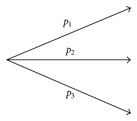
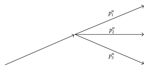
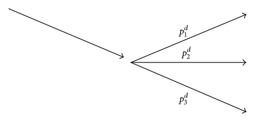
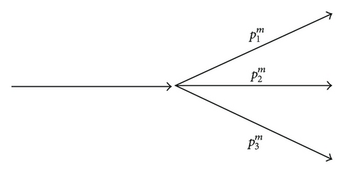
We remark that we think of as, respectively, risk-neutral versions of the empirical probabilities {p(u), p(m), p(d)} {p(u∣u), p(m∣u), p(d∣u)} {p(u∣m), p(m∣m), p(d∣m)} {p(u∣d), p(m∣d), p(d∣d)}.
Figure 1 will help us understand these complex probabilities.
Figure 2 is the trinomial tree established. Figure 3 is a trinomial tree with combination nodes and can be used to describe the movement of the stock price.
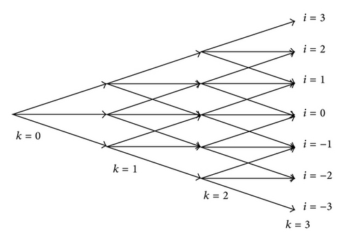
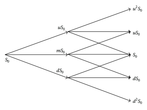
The calculating process of trinomial tree is similar to that of binary tree. It is pushing down option value from the tail of the tree to the root of the tree. The strike price and the value of holding the option are necessary to calculate at every node. By calculating, the value of holding the option is e−rt(Pufu + Pmfm + Pdfd).
When ;
When 1 ≤ k ≤ n1 − 1, for the quantity of the paths to reach each node in the trinomial tree, there are three possibilities: three paths, two paths, and one path. Here, we provide the formulas, respectively, for the three possibilities.
if the option is not a European option, but an American option. The calculation will be a little more complex. We should add a formula, which is (events means three different events u, m, d), besides (6).
Finally, we show the initial condition of the American call option.
3.1. Risk-Neutral Probabilities
For the character of the natural recombination, we set ud = m2 = 1. Compared with binomial tree, trinomial tree has the advantage of additional freedom degrees.
As a matter of fact, when we construct the trinomial tree to describe the change of the option price, it is to make the shape of the tree and the stock price volatility consistent, by choosing the value of P1, P2, P3.
Similarly, there are three volatilities σ+, σ=, σ− according to the three events, and risk-neutral probabilities can be calculated by formula (15).
Usually, we suppose .
If B2 < A, we suppose u = B2 + λ(A − B2), λ ∈ (0,1).
If C < B1, we suppose u = (1 + B1)/2.
Otherwise there are no reasonable risk-neutral probabilities.
3.2. Volatilities
For each date on which we wish to value an option, we start with the time series of one prior year’s worth of adjusted closing daily returns for the stock. We scan through this time series and form three disjoint time series: when In(Sn+1/Sn) > a, we add that return to series 1 (a is a threshold which is always greater than or equal to 0 and determines the market environment); when −a ≤ In(Sn+1/Sn) ≤ a, we add that return to series 2; when In(Sn+1/Sn)<−a, we add that return to series 3. We then take the logarithm of all returns in series 1, series 2, and series 3 and also in the original time series,
Set and l+ as the standard deviation and length of log return series, and set and l− as the standard deviation and length of log return series. Let be the standard deviation of the entire log return series. The standard deviations are, then, converted to volatilities σ, σ+ and σ− using and .
The parameters σ± are calculated precisely in the same way as σ, except that, for σ+, we take the standard deviation of log returns on days when the stock’s return increased, and the same way for σ− when the stock’s return decreased. This is discussed in greater detail above.
4. Comparison with Binomial Markov Tree
In the binomial Markov tree, when the number of states is large, the degree of efficiency of the tree models mentioned above is not high. But, in this paper, the proposed model is a combining tree, with the idea that under the first-order Markov process, we change the probability, the tree is still combining. Since it’s a combining tree, the nodes of the trinomial Markov tree are only 2n + 1 when k = n and its total node quantity are , while that of binomial tree is, respectively, n2 − n + 2 and . From this, it can be concluded that the computational complexity of trinomial Markov tree is ο(n2) while it is ο(n3) in the binomial Markov tree; on the other hand, for each node, the binomial Markov tree only has one value, but there is more than one value in the trinomial Markov tree which is decided by the path which comes to this node; that is to say, the computation of the proposed model is very fast and uncomplicated to implement.
What’s more, the path of the binomial Markov tree is more complex while using the backtracking method to handle. And it is very difficult in the programming application. However, because of the natural recombination, the trinomial Markov tree has its advantage, which can use the same backtracking method with the general trinomial tree, especially in American option.
In addition, there exists a weak point, in the binomial Markov tree; European option has the analytical solution which can be expressed by the formula. Yet the trinomial Markov tree perhaps has one but it is too complex to express.
5. Computing Case
5.1. Collecting Data
We estimate the risk-free rate using the no-arbitrage future pricing formula F = Sert, where F is the future price, S is the spot price, and t is the time horizon until expiration of the future contract. On August 24, 2009, we found that S = 75.43 and F = 75.658 for the AI future expiring in December 2009, which also gave t = 84 trading days = 0.33 years. This yields an annualized risk-free rate of r = 0.0090543.
We find that Air Liquide (Euronext: AI), a French company for estimating stock prices, uses data from August 25, 2008 to August 24, 2009. On August 24, 2009, we obtained it from euronext.com the end-of-day market prices for European call options of Air Liquide (symbol: AI) expiring in September 2010.
5.2. Convergence
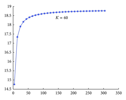
In Figure 4, x-axis is n1, and y-axis is the option price calculated. We can find from the figure that the value of European call option is increasing and convergent as n increases.
5.3. Sensitivity of Volatilities
Since the event that stock price remain the same from the day n to the day n + 1 is almost impossible in the actual market, in order to get a positive volatility of this event, we always let the volatility of district −a ≤ In(Sn+1/Sn) ≤ a as the volatility of this event. So we should make sure that the value of a (a is a positive constant greater than zero as described in Section 3.2) won’t affect the option price as possible as we can. If not, the trinomial Markov tree method is unreasonable, as we don’t know how to get a most reasonable a.
We will analyze the sensitivity of volatility when n = 100 as in Table 1.
| Strike | Market | B-S | Trinomial | a = 0.005 | a = 0.006 | a = 0.007 | a = 0.008 | a = 0.009 |
|---|---|---|---|---|---|---|---|---|
| 40 | 34.49 | 36.57 | 36.39 | 35.76 | 35.58 | 35.43 | 35.32 | 35.46 |
| 48 | 27.48 | 29.85 | 29.54 | 28.44 | 28.30 | 28.18 | 28.09 | 28.21 |
| 56 | 20.9 | 23.96 | 23.53 | 22.07 | 21.64 | 21.33 | 21.10 | 21.40 |
| 60 | 17.78 | 21.36 | 20.86 | 19.32 | 18.91 | 18.61 | 18.39 | 18.67 |
| 64 | 15.03 | 18.99 | 18.40 | 16.56 | 16.17 | 15.89 | 15.69 | 15.94 |
| 72 | 10 | 14.9 | 14.29 | 11.04 | 10.70 | 10.44 | 10.27 | 10.49 |
| 80 | 6.26 | 11.6 | 10.96 | 7.78 | 7.42 | 7.15 | 6.96 | 7.20 |
| 88 | 3.7 | 8.99 | 8.33 | 6.22 | 5.78 | 5.46 | 5.24 | 5.53 |
| 120 | 0.32 | 3.17 | 2.72 | 1.61 | 1.45 | 1.33 | 1.24 | 1.36 |
| 160 | 0.01 | 0.87 | 0.65 | 0.31 | 0.28 | 0.26 | 0.24 | 0.27 |
- Note: the first column is the strike price, the second is the market price, and the third is the price calculated by B-S model while the forth is calculated by the trinomial tree. The latter columns are the prices calculated by the proposed model when a is the corresponding value.
From Table 1, it can be found that as a increases, the option value doesn’t change much. It means that when calculating the option price with the method of trinomial Markov tree, we needn’t care much about how to choose a reasonable a.
The Markov trinomial tree model is tested against the ordinary trinomial tree model. From Table 1 we can see that option prices in Markov trinomial tree model are much closer to market prices than that in ordinary trinomial tree model when calculating ITM’ price (in-the-money options). However, it doesn’t show more superiorities than trinomial tree model when calculating out-of-the-money options.
The specific reason will be described in the sensitive analysis of u in Section 5.4.
5.4. Sensitivity of u
u = B2 + λ(A − B2), λ ∈ (0,1) have been described in Section 3.1; therefore, we can analyze the sensitivity of λ when n = 100.
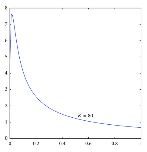
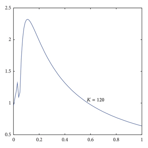
As seen from Figure 5, the option price has a small change as λ varies among (0.1, 1); that is to say, the sensitivity of u is weak. In other words, when calculating ITM, the option price stays stable no matter how λ changes among (0.1, 1). This is also the reason why option prices in Markov trinomial tree model are much closer to market prices than that in ordinary trinomial tree model.
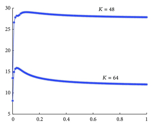
In Figure 6, x-axis is λ and y-axis is the option price calculated. It can spot from Figure 6 that the option price changes much as λ changes when λ is between (0,1). What’s worse, as the strike price of out-of-the-money option becomes higher and higher, the wave character becomes more and more obvious. That is to say, when calculating out-of-the-money option, the option price is not reliable due to its high sensibility unless we can find a method to determine a reasonable u. Therefore, we think that making u equal to is reasonable when calculating out-of-the-money options by numerical experiment.
6. Conclusions
We proposed a trinomial Markov tree for pricing options with recombining nodes. An algorithm for estimating the risk-neutral probability was given, and the condition of a validation risk-neutral probability existing was also provided. And then a method for estimating the volatilities was proposed. We analyze the convergence and sensitivity of the pricing method implementing trinomial Markov tree. Compared to binomial Markov tree, the proposed model is a natural combining tree; when changing the probability of the node, it is still combining, so we can draw the conclusion that the pricing method of trinomial Markov tree is very fast and very easy to implement.
Conflict of Interests
The authors declare that there is no conflict of interests regarding the publication of this paper.
Acknowledgments
This work is partially supported by NSFC (71273139), Chinese soft science (2010GXS5B147), the National public sector (weather) Special fund (GYHY201106019), the Department of philosophy and social science in colleges and universities in Jiangsu Province research Grants (09SJB630006), and the Priority Academic Program Development of Jiangsu Higher Education Institutions.


