Efficient UAV Path Planning with Multiconstraints in a 3D Large Battlefield Environment

1. Introduction

With the development of various modern high-maneuverability air defense weapons and increasingly perfected air defense system, the capability of vehicles to break through enemy defenses at medium and high altitudes has decreased. Modern military low-altitude penetration is primarily performed by UAVs. The key lies in the path planning for UAVs [1]. Research in this area has been ongoing for many years, and several algorithms were developed for this problem.

The artificial potential field method was developed by Khatbi to plan the trajectory for the robots. This algorithm is intelligible in its mathematical description and has been widely used for real-time obstacle avoidance and smooth trajectory control [2]. However, the method has its inherent limits when applied to UAV path planning [3]; for example, in complex mountainous terrains, there are often multiple obstacles near the target point; it would result in a greater repulsion than attraction for the UAV. Thus, the UAV cannot reach the target [4]. Some researchers hoped to establish a unified potential function to solve this problem [5]; unfortunately, it still requires regular obstacle to avoid huge calculation requirements, which is nearly intolerable for real-time path planning.

Some researchers have attempted to find the solution in intelligent optimization algorithms, such as genetic algorithm (GA) [6, 7] and ant colony algorithm (ACA) [8, 9]. The former has good global searching maneuverability and can quickly find all of the solutions without falling into local optimal [7]. The latter is highly robust and good at searching for better solution [8], and their experimental results present the feasibility to solve this problem. However, these algorithms have common limits that are difficult to avoid in solving large-scale UAV path planning problems. For example, genetic algorithm is weak for local search with low efficiency in the later periods and easily reaches premature convergence [6]. Ant colony algorithm is sensitive to the initial parameters. An inappropriate setting decreases the search rate and yields poor results [9]. Furthermore, the real-time path planning of UAVs requires high efficiency and accuracy; these algorithms may not be proper solutions.

Graph search algorithms have been developed to find the optimal trajectory between two nodes on connected graphs. The greatest advantage of these algorithms, including Dijkstra, Bellman-Ford, and A^* algorithms, is their straightforward implementation and low computational cost to get the optimal path, which makes it the most suitable method in theory [1]. The A^* solver is one of the most widely used algorithms among them. It was developed to analyze more effectively the domain in order to avoid distributed obstacles, which is largely applicable to robotics, space exploration, and video games [10]. Though maturely used in 2D graph searching, the A^* algorithm still faces some challenges in the UAV path planning in a 3D complex battlefield environment [11, 12], and previous research results may have problems as follows: (1) most experimental space was simple artificial topographies. The obstacles were few and regular, and complex threats such as radars and extreme weather conditions were not considered [13–15]; therefore, they did not verify their feasibility, efficiency, and convergence in large-scale complex space. (2) Some path planning is essentially performed in a 2D plane [16–18]. Some researchers use 2D spatial partitioning methods, like Voronoi map, to divide the target space into several sections to construct connected network graph. (3) The algorithms did not obtain a flyable path; most searching results are break lines or smoothing curves [14–17]. The maneuverability of the UAV, including the turning radius, safety altitude, climb rate, minimum step size, and fuel consumption, should be considered to get a flyable path, which is a fundamental difference from general robot path planning.

In light of the limitations above, the paper proposed an improved A^* algorithm for the UAV path planning in a 3D large-scale battlefield. This space is composed of real terrain data, radars, no-fly zones, and extreme weather conditions. The algorithm considers terrain following, threat avoidance, and fuel consumption to obtain a flyable path that follows the maneuverability constraints of a UAV. Meanwhile, an assessment algorithm was designed to evaluate the final path. Finally, the algorithm was compared with ACA and GA to present its advantage.

2. Materials and Methods

2.1. Modeling of the Battlefield Environment

The target space in this paper consists of a DEM map and battlefield plot information. Because the modeling methods for the former are very mature, this paper focuses on modeling the plot information, which includes radars, no-fly zones, and extreme weather.

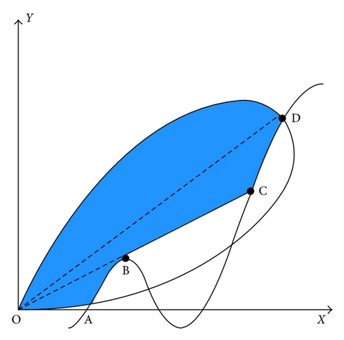
Radars have been widely used to detect the UAVs in modern air defense system. This paper does not treat radar like a normal obstacle but build a detection probability model, which distinguishes this research from most previous studies [19]. The process for computing the detection probability at any point in the target space is essentially the inverse of the radar equation and pattern function [20]. This value is calculated as follows.

(1) From the target point and radar antenna’s location, calculate the pitch angle, θ, and use the antenna pattern formula (1) to calculate the pattern function value F(θ) as follows:

$$ (1)

(2) Calculate the range from the target point to the radar center R(θ), and determine the maximum radar detection range R_max⁡. Consider

$$ (2)

(3) Invert the radar equation and the minimum SNR formula to determine the radar detection probability. The radar equation is shown in

$$ (3)

where P_av is the average transmitted power, G is the antenna gain, λ is the wavelength, σ is the radar cross section, k is the Boltzmann constant, T_m is the pulse recurrence period, t is the pulse length, T₀ is the absolute temperature in K, F_n is the noise figure of the receiver, B is the noise bandwidth of the receiver, L is the system loss factor, and [S/N]_min⁡ is the minimum SNR based on single pulse detection, which is defined as follows:

$$ (4)

where P_d is the detection probability, and P_f is the false alarm probability. We can obtain the detection probability P_d from formulas (3) and (4).

(4) Because modern radar normally adopts the standard of “M detections in N scans” [20], the detection probability, P, of any point must satisfy the following formula:

$$ (5)

This formula is nonlinear, so we can use the more efficient Newton iteration method [21] to determine the radar detection probability at any point in the target space.

Furthermore, we should also consider the influence of the terrain on the signal propagation; see Figure 1. Point O is the center of the radar antenna. If AB is the first mountain section, the area below BC is a blind zone because the beam is blocked by AB, and the final detection region in this section is the blue area between OABCDO. Figure 2 shows the radar coverage area ignoring the effect of terrain, while Figure 3 shows the real detection area. The real detection probability at any point is given by the following:

$$ (6)

where Z_R is the radar coverage and Newton is the Newton iteration method.

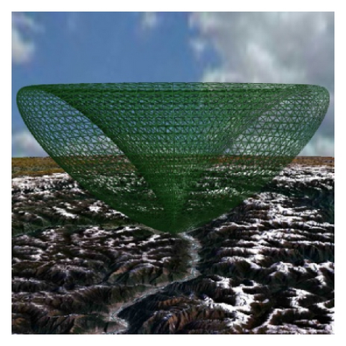
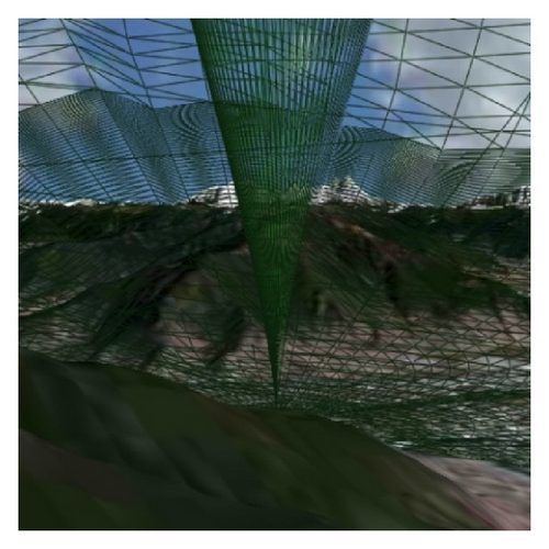
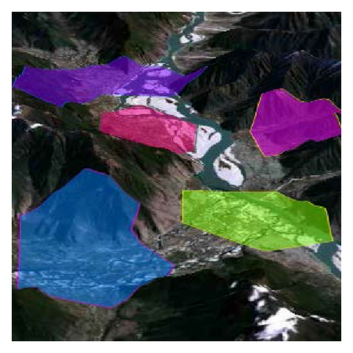
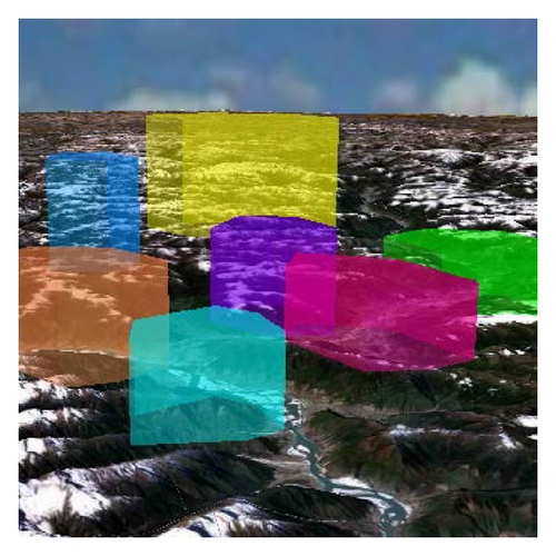
Extreme weather, including thunderstorms, blizzards, hails, hazes, and strong airstreams, poses a significant threat to the flight of UAVs. The climate threat model is divided into 2D and 3D zones based on its sphere of action. The former are described using a closed curve {P_i(x,  y)}, where x and y represent the longitude and latitude, respectively, and are shown in Figure 4. The latter are described using polygonal prisms ({P_i(x,  y)}, H_min⁡, H_max⁡). H_min⁡ and H_max⁡ are the altitude limits, respectively, and are shown in Figure 5. No-fly zones are described similarly to the 2D climate model.

2.2. Path Planning Strategies

2.2.1. Target Space Partition

The 3D area described by the DEM and DOM is a continuous raster space; therefore, there is no node-edge graph network present in traditional path searching, and spatial partitioning can solve this problem.

Some researchers used a Voronoi diagram to partition the space at a certain altitude [22]. Because UAVs change altitude during flight, this method is only applicable to certain flight missions in flat areas with small section changes at different altitudes. However, for mountainous terrain, this method cannot obtain a valuable optimal path. In addition, some researchers tried to use regular 3D boxes for the space partitioning [14]. It means that there are at least 26 nodes to expand during the searching process, which requires a large amount of time and memory to obtain an optimal solution, especially, in large space. This paper recommends a 2.5D partition model to solve this problem. The model is actually a surface partition model, which logically divides the DEM data into a series of independent rectangular grids in some accuracy. The terrain information in a grid is represented by its center. Each center point records the longitude, latitude, and altitude, as shown in Figure 6(a). The centers form a routing network needed in the routing process. This model has only 8 directions to expand for each node, which makes it more efficient than the 3D grid partition method.

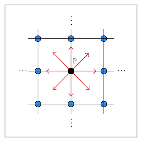
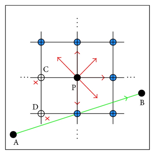
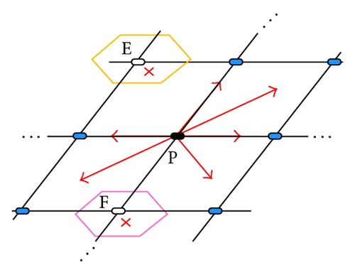
To further improve the convergence rate and efficiency of the algorithm, some researchers recommend considering the maneuverability constraints of UAVs [14, 17], including the minimum step size and turning radius, in nodes expansion. Satisfying the minimum step size requirement means increase of the grid size, which does improve the search speed to some degree, but it causes an excessive loss of terrain details and may greatly decrease the accuracy of the searching result. Considering the limits to the UAV’s speed, slope, and turning angle may decrease expansion directions, but some global optimal nodes may be missed due to the fact that the grid points are not the final waypoints. However, this method can be applied in local searching to filter out directions that the angle to the global direction is too large (e.g., >150°) as shown in Figure 6(b). In addition, this method can also filter out nodes in the no-fly zone and extreme climate threat as shown in Figure 6(c).

2.2.2. Initial Path Based on the Improved A^* Algorithm

The A^* algorithm cost function should be defined to evaluate the cost of the expansion nodes and obtain the node-edge list of the optimal path. The function is as follows:

$$ (7)

where n is the node being expanded, g(n) is the actual cost to from the initial node to node n, and h(n) is the estimated cost from node n to the target node. The heuristic function g(n) is the main factor affecting the search result, and a reference formula was made [23] to plan a terrain following path. Consider

$$ (8)

where c_t is the distance from a specified route, h is the altitude, f_TA is the threat value, and ω₁, ω₂, and ω₃ are their weights, respectively.

This heuristic function may have some problems when applied to the subject of this paper. First, c_t is a relative distance, but h is an absolute altitude, and they have differing magnitudes. The distance to the center of the threat, f_TA, is positively correlated with the cost function, and the lower this value is the better it is. However, c_t and h run counter to this value, which makes it not easy to assign a reasonable weight to each factor. Second, the threat of radar should be measured as a probability rather than a relative distance. Thus, it is several orders of magnitude lower than the other factors and the function would be too insensitive to ω₁, ω₂, and ω₃, which makes finding three values to develop a meaningful cost function for determining the optimal path difficult.

To solve the above problems, the cost function is improved as follows:

$$ (9)

In this formula, c_i is the surface distance from node i to node i − 1, which is the penalty for the route length. p_i is the detection probability between nodes i and i − 1 and is aimed at increasing the survival rate of the UAV. h_i is the weighted average altitude between nodes i and i − 1.

These three cost function factors all push in the same direction; that is, the solution requires a reduced route length, altitude, and detection probability. However, these factors are not on the same magnitude, and the penalty factors should be normalized. The key to adopting a 0-1 scale is to determine the maximum and minimum values for each factor. We cannot directly determine the maximum and minimum distance because it varies for each route segment due to the salient relief; however, regardless of the real or artificial terrain data, the maximum and minimum altitude is either already known or can be calculated from the data. Once h_max⁡ and h_min⁡ are determined, we can find the max and min of c_i; see as shown in Figure 7. Consider

$$ (10)

where $$ is the number of interpolation points between nodes i and i − 1 and d_i, Δh_i, and Δd are the Euclidean distance, altitude difference, and sampling interval, respectively.

p_i is the radar detection probability between nodes i and i − 1 and should be considered as the sum of all radars in the space. The corresponding formula is shown as follows:

$$ (11)

where p(R_j) is the weighted average probability of detection by the jth radar between nodes i and i − 1 for n_i interpolation points; the detection probability of each interpolation point can be calculated from formula (6). The normalization of these three factors is shown as follows:

$$ (12)

Formula (13) is the new cost function using these normalizations. In this formula, ω₁ + ω₂ + ω₃ = 1. Because the route length, altitude, and detection probability were normalized, the user can more directly assign the respective weights according to the planning objective. Consider

$$ (13)

In formula (7), h(n) was defined as the Euclidean distance from node n to the target point, which helps node n to approach the target point. Consider

$$ (14)

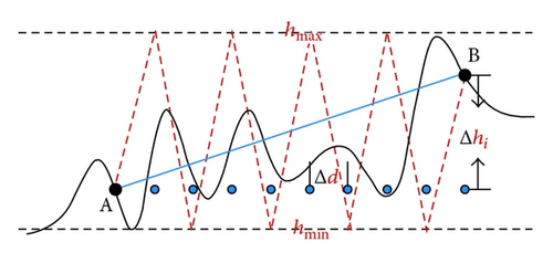
In this formula, d_n, d_max⁡, and d_min⁡ are the Euclidean, maximum, and minimum distances from node n to the target point as calculated using a similar formula to (10). However, it is worth mentioning that the sampling interval, ΔD, is generally greater than Δd to increase the efficiency of h(n).

Once the target space and cost function are set, the standard A^* path searching process can begin. Open and closed lists were defined to store the expanded nodes, which were implemented with the minimum binary heap and linear lists to increase the efficiency.

Furthermore, to compare the searching result in different parameters, formula (15) is designed to evaluate the final path as follows:

$$ (15)

where C is the route length, H is the mean altitude, and P is the detection probability. C_max⁡ and H_max⁡ are the maximum of C and H, respectively, and C_min⁡ and H_min⁡ are the minimum. ε₁, ε₂, and ε₃ are the weights of C, H, and P. Similar to the formula of g(n), a smaller value of V indicates a better path.

2.2.3. The Path Optimization Algorithms

The search results from Section 2.2.2 may not satisfy the UAV maneuverability constraints, such as minimum step size, turning radius, turning angle, climb rate, and safety altitude. Therefore, a series of algorithms are developed to obtain the final flyable path.

The minimum step size and turning radius are constraints on the top view. The former requires the length of each route segment to be above a certain value S_min⁡, while the latter requires every segment to be long enough for two continuous turns; therefore, we have to compress the initial route. To satisfy the two constraints, in this paper, the FFP algorithm is used for the data compression [24], and the longest rectilinear trend can be furthest preserved to avoid frequent turning of the UAV. In addition, the turning angle constraint requires every segment angle to be below a critical value, C_min⁡. A potential field algorithm can be developed to solve this problem [5]. As UAVs cannot fly along a broken line, some researchers recommend various curve smoothing methods such as the B-spline curve [25]. However, these methods obviously conflict with the minimum step size constraint. In fact, UAVs generally turn by escribing or flyby [26].

The climb rate and safety altitude are constraints on the vertical view. UAVs tend to maintain posture without frequent turns or climbs. If the altitude of two waypoints, A and B, is different, the UAV does not fly directly from A to B but first climbs to O from A at a certain climb rate before flying horizontally to B as shown in Figure 8. The safety altitude is the minimum distance from the ground to ensure safe flight. Because of various factors, like strong turbulence and automatic-control error, a UAV usually deviates from the predefined path. Therefore, the algorithm should consider the safety altitude across the entire deviation area. This area is the safety corridor of the path, and its mathematical model is shown in Figure 9 [26]. This corridor is divided into the primary and secondary areas with the former providing the entire safety altitude h and the latter providing safety between 0 and h. The safety altitude, Δh, at any point is calculated as follows:

$$ (16)

where h is the safety altitude, ΔL is the distance between the target point and the predefined path, and L is the width of the safety corridor.

Based on the mathematic models above, we propose the following algorithm to meet the safety altitude constraint between waypoint A and waypoint B.

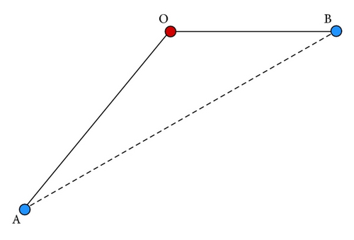
• (1)

  Divide AB into AO and OB, and O is the level-flight point calculated from the climb rate at A.

• (2)

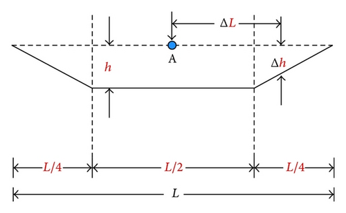
  Calculate the minimum signed altitude difference, ΔH₁, for the OB segment. Begin the spatial interpolation for OB to obtain a series of interpolated points, {P_i}. Divide the cross section of P_i into a primary area and two secondary areas, and calculate the corresponding minimum signed heights. Consider

  $$ (17)

•  

  where $$ is the minimum signed height difference for cross section P_i, h_B is the altitude of the OB segment, h is the entire safety altitude, Δh is the safety altitude of the secondary areas as calculated from formula (16), h_j is the altitude of the interpolation point j in the primary area, and h_k is the altitude of the interpolation point k in the secondary area. The minimum $$ value can be obtained by traversing {P_i}.

• (3)

  Calculate the minimum signed height difference, ΔH₂, of the AO segment. First, get the interpolation points, {Q_i}, between AO by spatial interpolation, and the minimum signed height difference for cross section i of Q_i is calculated by

  $$ (18)

•  

  where h_i = h_A + AO*(h_O − h_A)/AQ_i, and ΔH₂ can be calculated by traversing {Q_i}.

• (4)

  Adjust the altitude of O and B to h_B + ΔH₁ and the altitude of A to h_A + ΔH₂. Create a radial through A using the climb rate and calculate the intersection with OB, which is the new level-flight point O.

3. Results and Discussion

The test space was about 2,500,000 Km² between Linzhi in Tibet and Chengdu in Sichuan province and was constructed with SRTM terrain and LANDSAT image data in 30 m accuracy. The area is a mountainous district that can verify the feasibility and adaptability of the algorithms in this paper. The algorithms were developed with C# and Direct 3D, and they have been successfully used for a 3DGIS platform, Gaea Explorer [27]. The hardware environment was as follows: CPU: Intel Core2 Duo E8200, memory: Kinston 1 G, video card: ATI Radeon HD 2600 XT.

To prove the feasibility of the algorithms in this paper, we developed the parameters in Table 1. Before searching, we defined the UAV parameters in Table 2.

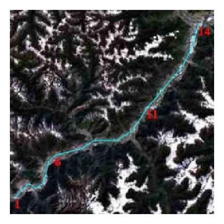
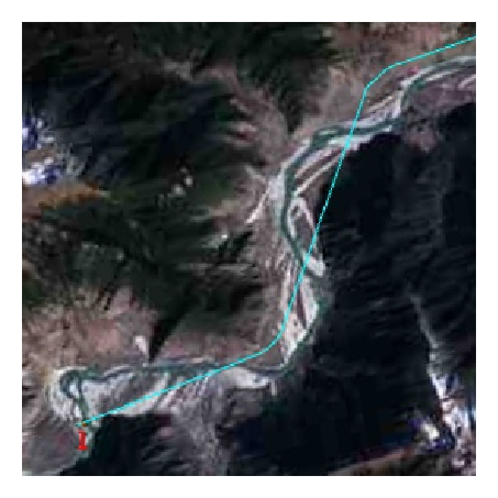
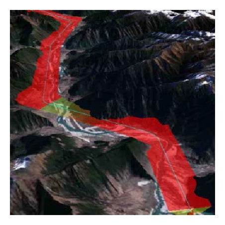
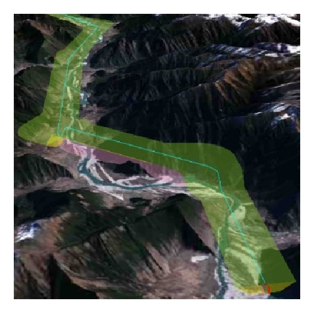
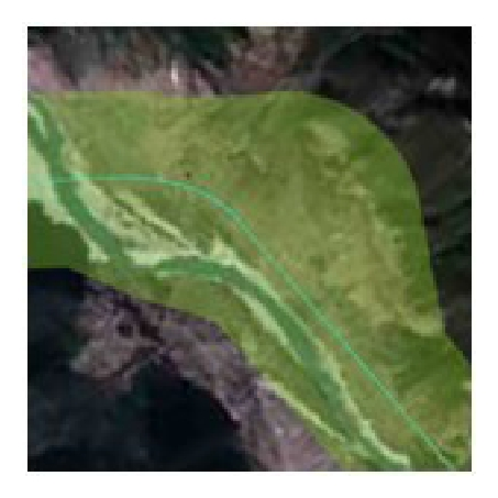
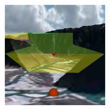
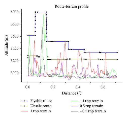
In Figure 10, (a) shows the initial search result, (b) shows the compression results, (c) shows the smoothing results, (d) shows the results that consider the climb rate, (e) shows the safety corridor result, (f) shows the results that consider the safety altitude, and both (g) and (h) show the local features of the safety corridor from the top and front views, respectively. To prove the safety of the final path, we calculated the profile at ±L/4 and ±L/2, as shown in Figure 11. From these results, we determined that the algorithms were effective for low-altitude UAV path planning.

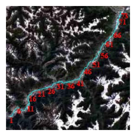
In Table 3, four experimental groups were designed to show the adaptability, convergence, and efficiency of the algorithm at various distances and grid sizes. Table 4 shows the parameters to evaluate the final path, where H_aver is the average altitude of the starting point and target point.

Table 5 shows that the algorithm can quickly determine the optimal path for various distances and grid sizes, which means that the algorithm is stable, convergent, and efficient. The time cost is proportional to the distance and inversely proportional to the grid size. Furthermore, the assessment value is smaller when the space partition grid is 0.01° rather than 0.005° or 0.02°.

To present the influence on the searching result of the changes of ω₁ : ω₂ : ω₃, the four groups in Table 4 were compared at the ratio of the weight factors ω₁, ω₂, and ω₃ being equal to 2 : 1 : 1, 1 : 2 : 1, or 1 : 1 : 1. The result in Table 6 shows that the time cost is proportional to the weight of the route length and inversely proportional to the weight of the route altitude. A higher weight of the length results in faster approach to the target point, but the UAVs would be more likely to be detected by enemies because higher nodes may be chosen in nodes extension. Considering the survival rate of the UAVs, a higher weight of the altitude may be more reasonable, and it was seemingly backed up by Table 6, which shows that the assessment value is the smallest when the weight ratio is 1 : 2 : 1 rather than 1 : 1 : 1 or 2 : 1 : 1.

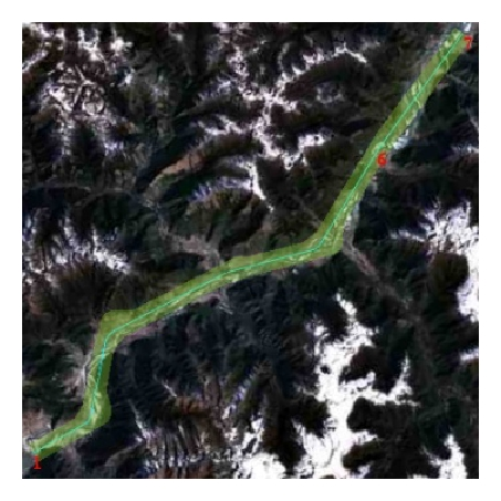
Figures 12(a)–12(d) show the results of the four comparison groups at a grid size of 0.01° and a weight ratio of 1 : 2 : 1.

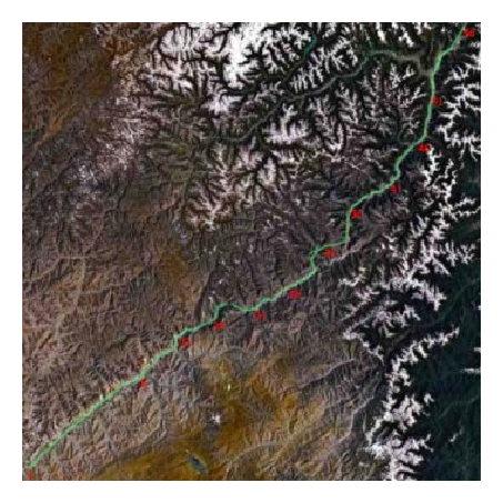
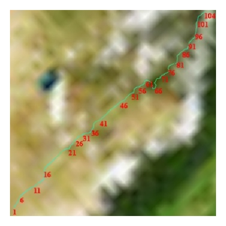
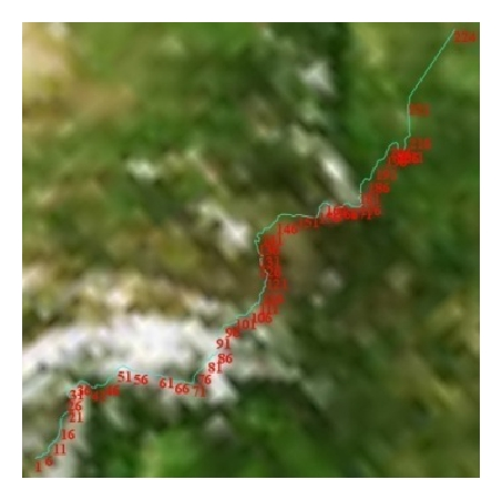
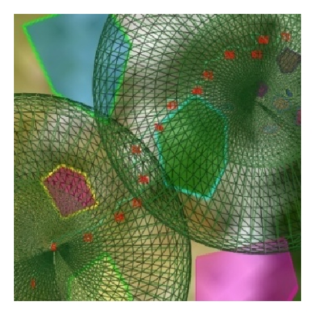
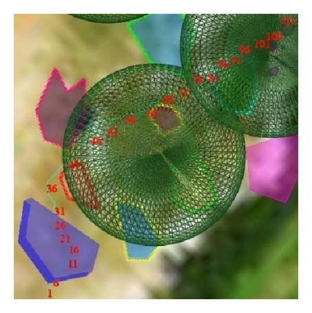
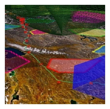
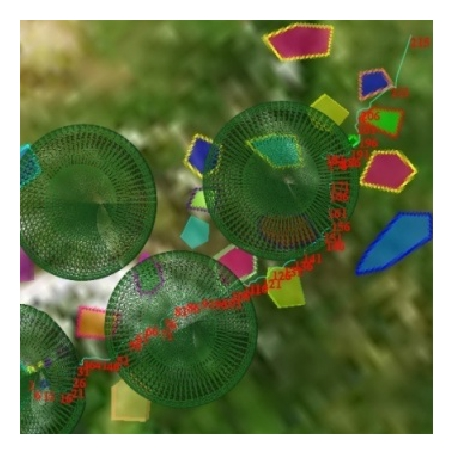
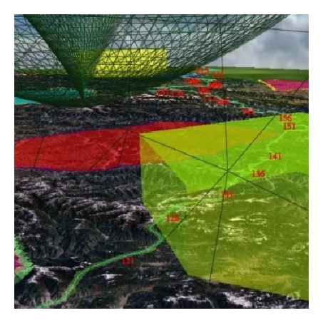
We created a battlefield environment of approximately 2,500,000 Km², as shown in Figure 13, to demonstrate the algorithm’s adaptability and convergence for large-scale complex situations including no-fly zones, extreme weather, and radars.

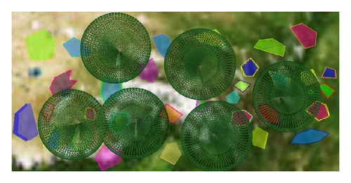
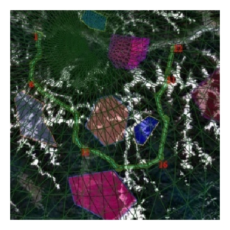
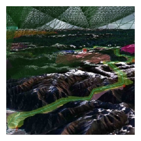
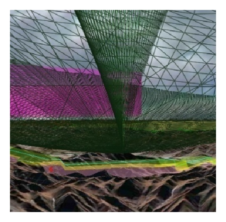
Table 7 shows the search results for the four groups at a grid size of 0.01°. The results prove that the algorithm is stable and convergent even for a complex battlefield environment. By comparing with the results shown in Table 4, we can see that the search time and route altitude increased slightly. Figure 14(a) shows the searching results for the first group; Figure 14(b) shows the local features. The other images are the results for the other three groups. These results indicate that the algorithm can effectively avoid no-fly zones and extreme weather while automatically searching for blind zones in radars network to accomplish a low-altitude penetration.

To present the advantages of the algorithm in solving the problem, we compared it with the ACA and the GA using the same parameters as in Table 3. The grid size is 0.001, and the iteration of ACS and GA is 2000.

The comparison results in Table 8 show that our algorithm has greater advantage in time efficiency than the other two algorithms, especially, in large scales, which is quite important in real-time path planning. On the surface, the advantage in the searching result is not so obvious, but the stability and convergence to get the optimal path still have comparative preponderance.

4. Conclusions

An improved A^* algorithm was developed for the path planning in large-scale 3D battlefields. The paper recommended a 2.5D spatial partition method for the 3D raster space, proposed a probability calculation model for radars network, and improved the A^* cost function to get an optimum route by considering the route length, the altitude, and the detection probability. A series of path optimization algorithms were developed to follow the maneuverability constraints of UAVs to obtain a final flyable path, and an assessment algorithm was designed to evaluate the path. The experimental results show that the improved A^* algorithm is stable, convergent, and efficient, and the comparison with ACA and GA shows its great advantage.

However, some issues should be further discussed. First, it is not so clear to quantify the planning goal to the optimal parameters, which is the key focus of decision makers. It was indicated that a comparatively good result was obtained at a grid size of 0.01° and a weight ratio of 1 : 2 : 1, but it is not easy to determine the exact optimal value of them. Table 6 presents that the path is better when the value of ω₁ : ω₂ : ω₃ is 1 : 2 : 1 rather than 1 : 1 : 1 or 2 : 1 : 1, but the assessment still depends on the parameters in Table 4.

Second, since the final path cannot be directly obtained by the A^* process as mentioned in Section 2.2.1., the searching result after the optimization process may no longer be the optimal solution. Although we adjusted the algorithms to locally optimize the route segments, globally optimizing the entire path is still to be solved.

Finally, the comparison of the improved A^* algorithm with ACA and GA shows its great superiority in time efficiency, but the advantage is not so obvious in the planning result, and more iterations of ACA or GA may even obtain better result than A^* algorithm. However, considering the internal limitations of the latter, like their stability (sensitive to initial parameters), convergence, and efficiency, they need to be further studied to be used in the UAV path planning.

Conflict of Interests

The authors declare that there is no conflict of interests regarding the publication of this paper.