A Numerical Test of Padé Approximation for Some Functions with Singularity
Abstract
The aim of this study is to examine some numerical tests of Padé approximation for some typical functions with singularities such as simple pole, essential singularity, brunch cut, and natural boundary. As pointed out by Baker, it was shown that the simple pole and the essential singularity can be characterized by the poles of the Padé approximation. However, it was not fully clear how the Padé approximation works for the functions with the branch cut or the natural boundary. In the present paper, it is shown that the poles and zeros of the Padé approximated functions are alternately lined along the branch cut if the test function has branch cut, and poles are also distributed around the natural boundary for some lacunary power series and random power series which rigorously have a natural boundary on the unit circle. On the other hand, Froissart doublets due to numerical errors and/or external noise also appear around the unit circle in the Padé approximation. It is also shown that the residue calculus for the Padé approximated functions can be used to confirm the numerical accuracy of the Padé approximation and quasianalyticity of the random power series.
1. Introduction
Padé approximation was introduced in mathematics by Hermite and Padé and it has been used in physics for more than 40 years ago [1–3]. In particular, there have been several important examples in physics, to which the Padé approximation was applied, such as summation of the divergent Rayleigh-Schrodinger perturbation series in scattering theory [4], critical phenomena in statistical physics [5–9], denoising from noisy data of time-series [10–14], and detection of singularity of phase space trajectories of Hamiltonian dynamical systems [15–19].
Mathematically, the Padé approximation can be used to estimate analyticity of functions. Indeed, the Padé approximation is usually superior to the truncated Taylor expansions when the original function contains any singularity. Let us consider a simple example. The function has brunch points at z = −1 and z = −1/2. The domain of convergence is |z | < 1/2. Nevertheless, we can obtain an exact solution √2 = 1.4142 for z → ∞ when we apply [3∣3] diagonal Padé approximation to the function (See Section 3.3 for more details on this example) Although the mathematical validity of the Padé approximation has not been exactly proved yet, the Padé approximation is practically very useful to continue a singular function beyond the domain of convergence.
In general, analytic continuation over the singular point is possible along any other path in complex plane even if the function diverges at the singular point determining the radius of convergence, as seen in the above singularity of the Ising model. Therefore, the Padé approximation is useful to improve the convergence of the power series and approximate the exact solution.
Furthermore, the Padé approximation has been used to investigate convergence of Fourier series [2, 3] and the breakdown of KAM curves in complex plane for Hamiltonian map systems, which is described as the analytic domains of Lindstedt series for standard map [15–19].
In addition, we can see an interesting example concerning the Padé approximation in noisy data analysis [10–14]. The power series with finite random coefficient “almost always” has a natural boundary on the unit circle in the complex plane [20–24]. In a finite time-series, Froissart has shown that a natural boundary generated by the random time-series is approximated by doublets of poles and zeros (Froissart doublets) of the Padé approximated function, which are surrounding the vicinity of the unit circle. Taking advantage of the characteristic, the Padé approximation has been used in order to remove the noise and extract the true poles associated with damping modes from the observed noisy time-series.
The main purpose of the present paper is to investigate whether the Padé approximation is numerically useful for detecting the singularity of some test functions. In particular, we examine the usefulness for the functions with a natural boundary such as a lacunary power series and a random power series [2, 13, 18].
The organization of the paper is as follows. In Section 2, we give a brief explanation of the Padé approximation and some important reminders in the numerical calculation. In Section 3, we present some numerical results of the Padé approximation for test functions with branch cut, essential singularity. We also try to apply the Padé approximation to an entire function. In Section 4, application of the Padé approximation to some lacunary series which is known to have a natural boundary is given. In Section 5, numerical results of the application to random power series with a natural boundary and some test functions with random noise are also shown. In Section 6, we discuss the residue calculus for the Padé approximated functions to confirm the numerical errors and quasianalyticity of the random power series. In the last section, we give summary and discussion.
In Appendix A, the general result for Fibonacci generator used in Section 3.2 is given. In Appendix B, some theorems concerning zeros of polynomials are given. In Appendix C, some mathematical theorems for lacunary series, which are useful in reading the main text, are summarized. In Appendix D, exact Padé approximated functions to some lacunary power series with a natural boundary are given. Residue analysis for quasianalytic functions of Carleman class is given in Appendix E. Furthermore, some theorems concerning the random power series are given in Appendix F.
2. Padé Approximation
In this section, we give preliminary instructions to the Padé approximation and some important reminders on the numerical calculation.
Generally, the magnitude of the residues associated with the spurious poles is much smaller than that with the true poles, and they are close to machine precision. Very recently, Gonnet et al. suggested an efficient algorithm for the Padé approximations [30, 31]. The algorithm detects and eliminates the spurious pole-zero pairs caused by the rounding errors by means of singular value decomposition for the Teoplitz matrix.
- (1)
More accurate calculation becomes possible by scaling the expansion variable z if there is a simple pole with large magnitude ρ(≫1). That is, we should change the order of radius of convergence into O(1) by the scaling the expansion variable as z → z/ρ in order to keep the numerical accuracy. This procedure is effective when we apply the Padé approximation to exponentially decaying coefficients {an} with fluctuation.
- (2)
Poles (i.e., roots of PM(z) = 0) and zeros (i.e., roots of QM(z) = 0) are sometimes cancelled (zero-pole ghost pairs). We can remove the effects of the ghost pairs and confirm the singularity of the functions by using the residue analysis of the Padé approximated function.
- (3)
Poles and zeros of the Padé approximation to the truncated random power series accumulate around the unit circle as Froissart doublets. It is difficult to distinguish whether the poles of the Padé approximation originated from a natural boundary of the original function or the natural boundary generated by the numerical error and/or noise. Therefore, the numerical accuracy will be important to determine the coefficients of the Padé approximation.
- (4)
In general, the denominators of the diagonal Padé approximated functions to the lacunary power series and the random power series become lacunary and random polynomials, respectively. Accordingly, the distribution of the poles and zeros of the approximated functions are similar to the distribution of the zeros corresponding to the original lacunary power polynomial and random power polynomial. In particular, it is well known that the zeros of the random polynomials uniformly distribute about the unit circle (see Appendix B).
3. Examples of Padé Approximation for Some Functions
In this section we investigate the configuration of the poles and zeros of the Padé approximation to some test functions with singularity.
3.1. Comparison of Padé Approximation with Taylor Expansion
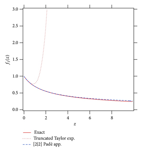
Figure 1 shows the approximated functions, the truncated Taylor series , and the original test function f1(z). The approximated function by the truncated Taylor expansion converges only within |z | < 1 and deviates from the exact function f1(z) for |z | > 1. On the other hand, it follows that the Padé approximated function well approximates the original function f1(z) with very high precession even beyond the radius of convergence up to Rez = x ~ 10. Therefore, it is found that the divergent power series expansion (Taylor expansion) does still contain information about the original function outside the convergence radius, and rearranging the coefficients of the expansion into the Padé approximation recovers the information. As a result, the conversion from the Taylor form to the Padé form usually accelerates the convergence and often allows good accuracy even outside the radius of convergence of the power series.
3.2. Padé Approximation for Fibonacci Generating Function
3.3. Examples of Some Test Functions with Pole, Brunch Cut, and Essential Singularity
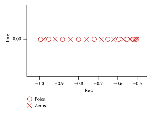
In Figure 2(b), distribution of the zeros and poles of the Padé approximated function to f3(z) is shown. The poles and zeros make a line alternately between the two branch points of the f3(z); z = −1 and z = −1/2.
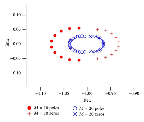
Figure 2(c) shows the distribution of the zeros and poles of the Padé approximation to f4(z). The Padé approximation clusters the poles and zeros at the singular point for f4(z). As M → ∞ the poles and zeros approach the singular point z = −1 that reflects the essential singularity of the original function f4(z).
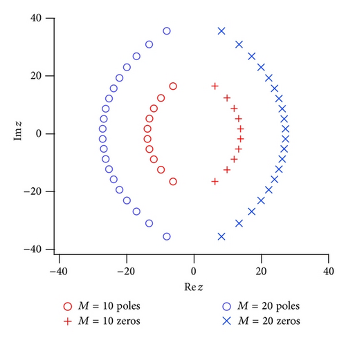
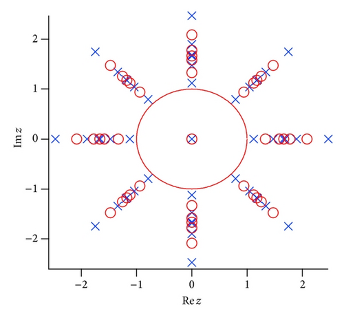
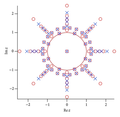
Figure 3(a) shows the poles and zeros of the Padé approximated function to the test function f5(z). The poles and zeros are alternatively distributed in eight directions from the origin. It seems that the distance between the poles and/or zeros on the same line becomes small as they approach the location of the true poles. Some “spurious poles” appear around the unit circle with the increase of the order of the Padé approximation, as seen in Figure 3(b), which are irrelevant poles due to insufficient numerical accuracy. It is found that the numerical accuracy of the Padé approximation fails for the higher order of the Padé approximation. We discuss the spurious poles in Sections 4 and 5 again.
4. Natural Boundary of Lacunary Power Series
In this section, we examine the applicability of the Padé approximation to investigate the analyticity of some well-known test functions with a natural boundary on the unit circle |z | = 1. This will provide a preliminary information about what occurs in the Padé approximated functions for some test functions with a natural boundary. Indeed, we do know only a very few numerical examples which have a natural boundary and allow an exact diagonal Padé approximation.
The following are famous lacunary power series with a natural boundary on the unit circle |z | = 1, , , and , where the fJac(z), fWie(z), and fKro(z) are called after Jacobi, Weierstrass, and Kronecker. Some theorems for the lacunary series with a natural boundary are given in Appendix C [20–22].
4.1. Example 1: Jacobi Lacunary Series
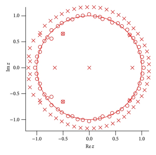
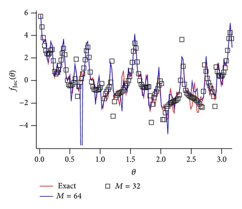
It is also shown that the complex zeros of the polynomial (17) cluster near unit circle |z | = 1 and distribute uniformly on the circle as FN → ∞ by Erdos-Turan-type theorem given in Appendices C and B [34–41].
4.2. Example 2: Fibonacci Lacunary Series
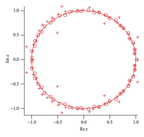
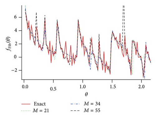
In Figure 5 the numerical result of the Padé approximation to fFib(z) is shown. The poles and zeros are plotted for the [55∣55] Padé approximation in Figure 5(a). The poles and zeros accumulate around |z | = 1 with the increase of the order of the Padé approximation. No pole appears inside the unit circle. The original function is also well approximated by the [56∣56] Padé approximation (see Figure 5(b)).
5. Natural Boundary of Random Power Series and the Noise Effect on Padé Approximation
In this section, we apply Padé approximation to the random power series with a natural boundary with probability 1 and investigate how the approximation detect the singularity of the series. In addition, we examine the effect of noise on the coefficients of the power expansion for some test functions. Some related theorems for the natural boundary of the function generated by the random power series are given in Appendix F.
5.1. Random Power Series and Natural Boundary
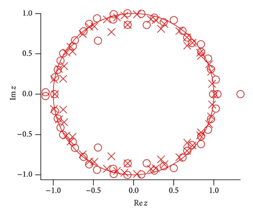
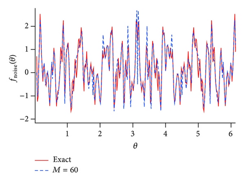
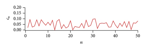
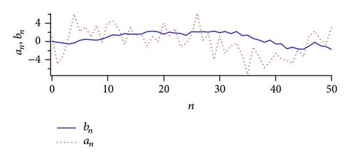
Figure 7 shows an example of the coefficients {cn} = {ϵrn} of the random power series and the coefficients {an} and {bn} of the [50∣50] Padé approximated function. The fluctuation of the coefficient {bn} that determines the poles of the Padé approximated function is smaller than that {an} of the numerator.
Note that the truncated random series is a random polynomial. As for the random polynomial, it is well known that the distribution of the zeros converges on the unit circle when the order of the random polynomial increases (Erdos-Turan-type theorem) [34, 35, 40]. Accordingly, we can generally interpret that in the Padé approximated function to the random power series the distribution of poles and zeros also accumulates around the unit circle when the order of the Padé approximation increases. The dependence of the zeros of the random polynomial and the zeros and poles of the Padé approximation has been studied by Gilewicz and Kryakin [42] and Ding and Xiao [43].
5.2. Effect of Noise on a Function with a Simple Pole
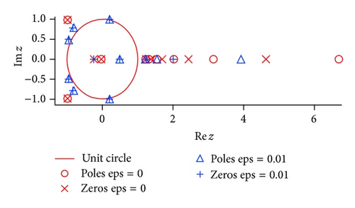
Figure 8 shows distribution of the poles and zeros of the [10∣10] Padé approximated functions. It clearly shows the pole shift by the noise effect. In the noise-free case (ϵ = 0), a pole of the Padé approximation appears at z = 2 and the other poles are cancelled with zeros (zero-pole ghost pairs). In a case when the relatively small noise (ϵ = 0.01) is added, the poles and zeros move toward |z | = 1 with making Froissart doublets, although a pole at z = 2 is quite stable. It becomes impossible to detect the true pole at z = 2 when the noise strength is relatively large (ϵ = 0.1), not shown in Figure 8.
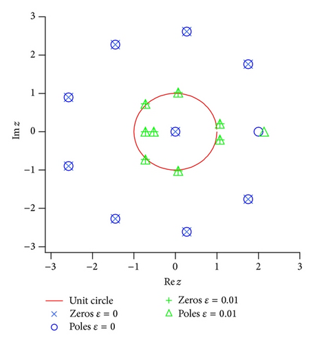
As a result, it is found that the locations of the ghost pairs are unstable for noise, and the residues for the poles are much smaller than one corresponding to the true pole. We can guess that the proximity of the nonmodal poles and zeros of the Padé approximated function can be understood in a sense that the poles due to the noise need zeros to cancel with each other as ϵ → 0.
5.3. Effect of Noise on a Function with a Branch Cut
5.4. Effect of Noise on a Function with a Natural Boundary
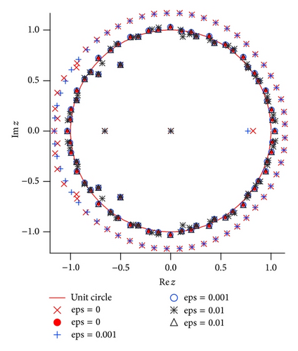
In the noise-free case, the pairs of poles and zeros of the Padé approximated function are perfectly cancelled inside the unit circle |z | = 1. The other poles and zeros of the Padé approximated function assemble around the circle |z | = 1 without cancellation. In the relatively small noise case (ϵ = 0.01), the location of the poles is not significantly changed compared with the zeros shifted outside the unit circle due to the noise effect. And, again, the poles and zeros move toward |z | = 1 with making Froissart doublets when the noise strength is relatively large (ϵ = 0.1). It is closely related to a fact that fluctuation of the coefficients of the numerator of the Padé approximated function is much larger than those in the denominator, as seen in Padé approximation to the random power series in Figure 7. As a result, the singularity of the Padé approximated function for the function with a natural boundary is more sensitive to the noisy perturbation than that in the functions with the other type singularity such as simple poles and branch points.
It is very difficult to effectively distinguish whether the poles of the Padé approximation originated from the natural boundary on |z | = 1 of the original function fJac(z) or from the other natural boundary on |z | = 1 generated by noisy series fnoise2(z) or numerical errors. Actually the round-off error affects the distribution of the poles and zeros of the Padé approximated function. Accordingly, to determine the expansion coefficients cn with adequate accuracy becomes very important in the numerical calculation. This is a drawback of the Padé approximation when we use it for functions with unknown singularities.
5.5. Numerical Accuracy and Spurious Poles
As we observed in the last subsection, the effect of rounding error and accuracy limit of computers work in the numerical results of the Padé approximation. As the result of accumulation of the round-off error, the “spurious poles” appear around the unit circle |z | = 1 as the pole-zero pairs when the order of Padé approximation increases (we used a term “Froissart doublets” for the poles-zero pairs generated by random power series, conveniently, although we cannot numerically distinguish it from the spurious poles due to the round-off errors; in the next section, we will discuss the Froissart doublets again).
However, we can roughly distinguish between true poles and the spurious poles by “residue analysis” of the Padé approximated function because the spurious poles-zero pairs are unstable for the change of the order. In this subsection, we try to investigate the residues of the Padé approximation for some test functions. Up to now, the residue analysis has been mainly used for performance comparison between the different algorithms of the Padé approximation of the same order [30, 31]. On the other hand, it seems that the study by using the information of the residue analysis is still rare in the Padé approximation [10, 12].
Here, we investigate the convergence property of the magnitude of residues |Ak| arranged in descending order.
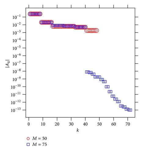
Figure 12 shows the absolute value of the residues |Ak| of some Padé approximated functions for the test function f5(z), which are arranged in descending order (note that they are noise-free cases.) The distribution of the poles and zeros of the Padé approximated functions is given in Figure 3. In a case of M = 50, the magnitude of the all residues |Ak| is larger than O(10−3), which correspond to the relevant poles arranged radially in eight directions from the true poles. On the other hand, in a case of M = 75, the spurious poles appear and distribute around the unit circle |z | = 1 (see Figure 3(b)). It is found that the absolute values of the residues corresponding the spurious poles are several order of magnitude smaller than the relevant poles.
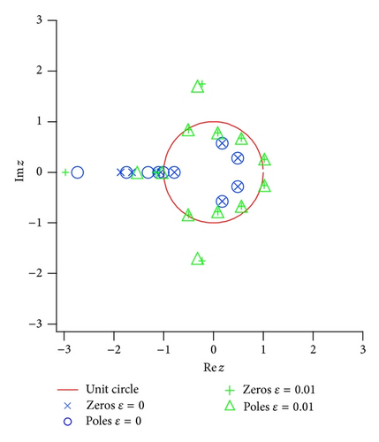
Distribution of poles and zeros of the Padé approximated function for the test function fbranch2(z) is shown in Figure 13. The stable poles and zeros are lined on [6/5, ∞], and the spurious poles appear around |z | = 1. The magnitude of the residues of the spurious poles is also enormously small compared with that of the stable poles remaining with the increase of the order of the Padé approximation.
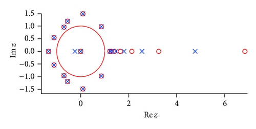
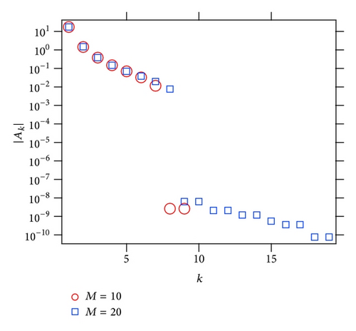
Figure 14 is also the result of the residues analysis for the Padé approximated function for the test function fJac(z) with a natural boundary on the unit circle |z | = 1. In the [50∣50] Padé approximated function, the magnitude of the residues |Ak| is shown in changing the noise strengths ϵ = 0,0.01,0.1 corresponding to poles-zeros distribution in Figure 11.
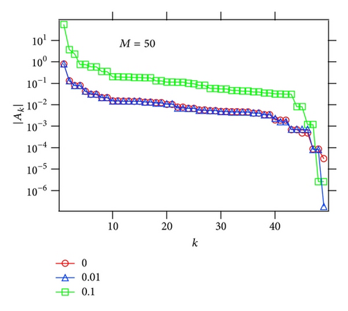
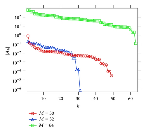
In the small noise case (ϵ = 0.01), the results of the residue analysis for fJac+noise2(z) is almost the same as the noise-free case (ϵ = 0), and in the case with relatively strong noise (ϵ = 0.1), the noise shifts the magnitude of the residues with larger value. In addition, the result of the residue analysis of the noise-free cases for some different orders of the Padé approximation is shown in Figure 14(b). We should have in mind that the order is important when we apply Padé approximation to the lacunary power series because we should not take the order of the approximation in the gap of the series.
6. Froissart Doublets
The problem of constructing the Z-transform Z(z) of a finite time-series is a standard problem in mathematics [10–14]. For example, it is shown that for a sum of oscillating damped signals, the Z-transform associated with the time-series can be characterized by a sum of the poles of the Padé approximated function. The position of each pole is simply linked to the damping factor and the frequency of each of the oscillators. Also, it is important to note that all these poles lie strictly outside the unit circle because it corresponds to the damping [10–13]. In addition, we will consider quasianalyticity property of the random power series by the residue analysis of the Padé approximation.
6.1. Noise Attractor
On the other hand, let us consider a noise-added sequence {S0, S1, …, Sn, …}. Then, the Froissart pointed out that there are two types of the poles: stable poles and unstable poles when we apply the diagonal Padé approximation to the unknown data set. In general, the Z-transform of the noisy sequence has a natural boundary on the unit circle |z | = 1 with probability 1. In fact, the poles and zeros (Froissart doublets) of the Padé approximated function often distribute around the unit circle when the numerical error and/or noise are mixed into the Taylor series of the analytic functions, as seen in the last section. That is to say, we sometimes call the unit circle |z | = 1 noise attractor in a sense that the poles and zeros are attracted to the circle as the Froissart doublets [45]. Accordingly, it is found that Padé approximated function for the function Z(z) has stable poles associated with the damping modes and unstable spurious poles associated with the noisy fluctuation. After elimination of the spurious poles around the noise attractor from the noisy sequence we can reconstruct the noise-free sequence consisting of the stable poles located in the domain |z | > 1. Another remarkable feature of the nonmodal poles is that the absolute values of the Cauchy residues associated with them are usually much smaller than those associated with true poles.
6.2. Random Power Series and Quasianalytic Function
Weierstrass defined the analytic function by direct analytic continuation of function. Then, apparently the analytic continuation is impossible beyond the natural boundary even if we can uniquely define the function and it is analytic outside the analytic domain. Borel and Gammel extended the narrow condition for the analyticity and gave a definition of quasianalytic functions [46, 47]. Gammel conjectured the following for the random power series [10, 45].
Gammel-Nuttall Theorem (1973). If Bk in (33) satisfies the condition (34) and |ωk | = 1, then the sequence of [N + J∣N] Padé approximation to the fGammel(z) converges in measure to the function fGammel(z) as N → ∞ in any closed, bounded region of the complex plane, where J is a natural number that equals N or less.
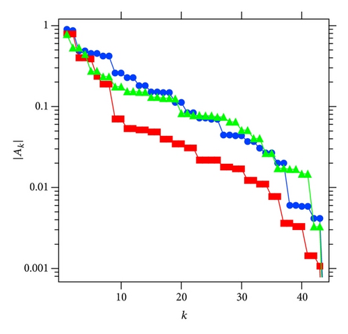
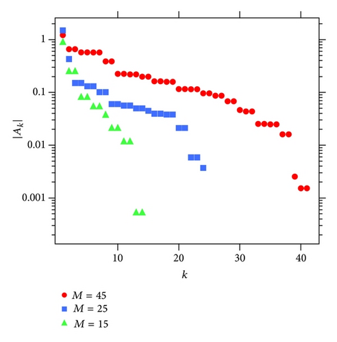
However, it is not nearly so simple. We should check the stability of the exponential-like decay of the magnitude of the residues by changing the order of the Padé approximation. Figure 16 shows the result for the three different orders: M = 15, M = 45, and M = 55. It expresses an indication that the decay exponent β does not converge to a positive certain value. It seems that the exponent behaves β → 0 as a limit M → ∞. On the other hand, if we directly apply the Padé approximation to the quasianalytic function fGammel(z) with Bk = e−k, the exponent β is stable for changing the order of the Padé approximation (see Appendix E). These facts suggest that the random power series does not belong to Carleman class of quasianalytic functions although it has a natural boundary on the unit circle, and it has the form (33). As a result, we can say that no optimism is warranted on the Gammel conjecture.
How does the residue analyses of the Padé approximation for the analyticity and/or quasianalyticity of unknown function work? It is an interesting and future problem.
7. Summary and Discussion
In the present paper we numerically examined the effectiveness of the Padé approximation for some test functions with branch point, essential singularity, and natural boundary by watching the singularities of the Padé approximated functions. For the functions with a branch cut, the poles and zeros of the Padé approximated function are lined along the true branch cut. The poles and zeros are distributed around the true natural boundary if the original test function has a natural boundary. In addition, we gave the explicit Padé approximated functions for some lacunary power series which are useful to check the numerical result. It was shown that, in particular, the distribution of poles and zeros of the Padé approximated function for lacunary power series and the random power series accumulated around the unit circle when the order of the approximation increases.
We often suffer from the difficulty to distinguish whether or not the poles of the Padé approximation are intrinsically originated from the natural boundary of the original power series because the numerical errors contained in the expansion coefficients also yield a false natural boundary. Therefore, the expansion coefficients with adequate numerical accuracy are necessary when we apply the Padé approximation to functions with unknown singularities.
Furthermore, the residue calculus of the Padé approximated function is useful when we detect the singularity of the original power series from the asymptotic behavior of the truncated series. It is useful also for estimating the accuracy of the approximation. As a result, the residue calculus suggested that the random power series does not obey Gammel’s conjecture; that is, it does not belong to Borel class of the quasianalytic functions.
We finally remark that the most serious problem to be improved is the numerical accuracy due to the limitation of the order in the Padé approximation when we use it for detecting unknown singularities of wave functions in quantum physics [32].
Conflict of Interests
The authors declare that there is no conflict of interests regarding the publication of this paper.
Acknowledgments
This paper was partially written for “International Symposium of Complexified Dynamics, Tunnelling and Chaos” held on 2005 in Kusatsu. This work is partly supported by Japanese people’s tax via MEXT, and the authors would like to acknowledge them. They are also very grateful to Dr. T. Tsuji and to Koike Memorial House for using the facilities during this study.
Appendices
A. General Recursion Relation
It becomes Fibonacci sequence when we set a0 = 0, a1 = 1, and ak = ak−1 + ak−2.
B. Random Polynomial
The following theorems concerning the random power series are well known.
Note that this theorem also holds for the polynomials with deterministic coefficients an such as Newman-type polynomial having coefficients in the sets {0,1} or {0, ±1}.
C. Some Gap Theorems of Lacunary Power Series
D. Numerators of Diagonal Padé Approximations for fJac(z) and fFib(z)
We have inductively obtained above results by means of Mathematica.
E. Residue Analysis for Carleman Class of Quasianalytic Functions
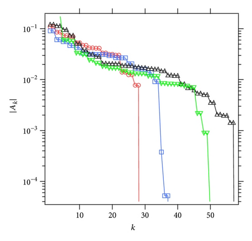
As a result, it seems that |Ak| exponentially decreases with a stable exponent, regardless of the order of the Padé approximation. This supports that certainly, the Padé approximation is applicable to the quasianalytic functions in the Gammel conjecture as given in Gammel-Nuttall theorem. The Padé approximation for the quasianalytic function converges to the function even outside the unit circle. It should be also noted that in all cases the tails of |Ak| are rapidly decay because the “truncated” series are essentially analytic functions.
F. Some Results for Natural Boundary in Noisy Series
In this appendix some theorems for the random power series are given. See, for example, [21] for the proofs.
The similar theorems can hold for random power series with a sequence of stochastic variables obeying i.i.d. in the interval ri ∈ [−1,1] or ri ∈ [0,1] [48].
Kahane’s Theorem (1985). The circle of convergence is the natural boundary for random Taylor series (F.1) if the coefficients {an} are independent and symmetric random variables.
The more generalized version has been given in the following form [22].
Breuer-Simon Theorem (2011). Suppose that the power series (F.1) has the convergence radius 1. Then for a.e. ω, has a strong natural boundary on |z | = 1 if the an(ω) is a stationary, ergodic, bounded, and nondeterministic process.


