Exact Inference for the Dispersion Matrix
Abstract
We develop a new and novel exact permutation test for prespecified correlation structures such as compound symmetry or spherical structures under standard assumptions. The key feature of the work contained in this note is the distribution free aspect of our procedures that frees us from the standard and sometimes unrealistic multivariate normality constraint commonly needed for other methods.
1. Introduction
In general, research and testing methods of this form assume an underlying multivariate normal distribution with associated exact and approximate tests; for example, for a thorough overview and history of this testing problem, see Seber [1] and the references therewithin. In practice one can safely say that it would be rare that the multivariate normality assumption holds. Hence, we were motivated to develop an exact permutation method approach to this problem. To the best of our knowledge no so-called exact permutation tests have been developed or explored with the exception of the very special case of p = 2 dimensions and testing H0 : ρ12 = 0; for example, see Good [2]. Martin [3] provides a bootstrap algorithm for testing H0 : ρ12 = ρ12,0, which asymptotically can be shown to have the appropriate type I error rate. Unfortunately, the bootstrap methods given by Martin [3] relative to first standardizing the variables and rotating the data so as to transform the problem to the setting of testing H0 : ρ12 = 0 do not work in the permutation setting. The permutation test for the case H0 : ρ12 = 0 follows by permuting the second column of the n × 2 data matrix (X1, X2) and calculating the test statistic , where refers to the standard sample Pearson correlation coefficient, over all permutations. This can be done directly via a computationally expensive algorithm or via the more widely used Monte Carlo techniques. With respect to the Monte Carlo methods we generate B random permutations of the data and denote the permuted value of the test statistic by . Then the one-sided P value for the alternative H1 : ρ12 > 0 is given as , where the index i corresponds to a given permutation and I denotes the indicator function. Alternative approaches found in software packages such as SAS PROC FREQ (SAS version 9.3, Cary, NC) utilize hypergeometric probabilities similar to how Fisher’s exact test is carried out via treating the fixed data as discrete.
In general permutation testing is most often used for comparing two groups in the context of location differences or other features of distributions such as scale measures. Most of the theoretical work has been done in this setting such as type I error control. For a technical treatment of permutation testing see Romano [4] with respect to a theoretical examination for the behavior of the type I error control for permutation tests under exchangeability versus nonexchangeability conditions. In order to ensure true bounded type I error control in the permutation testing setting either the null hypothesis has to be specified in such a way that exchangeability holds by definition under H0 or some design feature such as randomization or matching needs to be employed. Commenges [5] studies the more general transformation approach used to preserve exchangeability. Also, see Zhang [6], Huang et al. [7], and Janssen and Pauls [8] with respect to the inflation of type I error rates when comparing means in the two-sample setting along with other types of comparisons. In terms of permutation testing related to correlation structure based hypotheses very little has been accomplished. This paper represents one of the only investigations of this type to date.
In Section 2 we develop the general p-dimensional exact tests given a prespecified covariance structure. Special cases include testing for sphericity, compound symmetry, and block diagonality, to name a few. This presentation is followed by a simulation study in Section 3. We then apply our method in Section 4 to an example involving repeated measures mice weight data.
2. Exact Tests for Covariance Structures in p Dimensions
The focus of the work in this setting is with respect to two-sided alternatives. In certain instances a subset of these tests with one-sided alternative structure may be constructed. Those tests will not be included as part of this discussion due to the specificity of their applications.
2.1. Unequal Variance Setting
- (1)
Define H0 at (5).
- (2)
Obtain the new random variates Z by applying the transformation to the observed data X.
- (3)
Calculate T(Z) at (7).
- (4)
Permute each column of Z independently such that we have the permuted n × p matrix denoted by Z*.
- (5)
Calculate T(Z*) applying the resampled values to T(Z) at (7).
- (6)
Repeat steps (4) and (5) B times.
- (7)
Calculate the Monte Carlo estimated permutation P value as , where I(·) denotes the indicator function.
2.2. Nontransformation Special Cases
2.3. Equal Variance Setting
- (1)
Define H0 at (15).
- (2)
Obtain the new random variates Z by applying the transformation to the observed data X.
- (3)
Calculate T(Z) at (7).
- (4)
Permute each column of Z independently such that we have the permuted n × p matrix denoted by Z*.
- (5)
Calculate T(Z*).
- (6)
Repeat steps (4) and (5) B times.
- (7)
Calculate the Monte Carlo estimated permutation P value as , where I(·) denotes the indicator function.
A special case relative to testing hypothesis (15) is the test that the dispersion matrix is diagonal and all , i = 1,2, …, p.
- (1)
sphericity:
() - (2)
compound symmetry:
() - (3)
first-order autoregressive:
() - (4)
spatial power:
()
Several other well-known spatial dispersion matrices similar to the spatial power matrix presented above fit within this same framework and will not be presented here.
3. Simulation Study
- (1)
compound symmetry:
() - (2)
first-order autoregressive:
()
Note that the special case ρ0 = 0 is the same for both covariance structures and is only presented once. It should also be noted that under the assumption of multivariate normality testing H0 : Σ = σΓ0(0) under the compound symmetry or first-order autoregressive structure is a special case (equal variance assumption) of the well-known test for “complete independence”; for example, see Mudholkar et al. [9]. Under nonnormality we are essentially testing the “complete uncorrelated” case. In this special case the methods presented here are the first exact methods developed for tackling this particular hypothesis. In terms of large sample theory around similar results see Jiang [10] and Xiao and Wu [11].
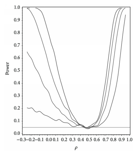
For our simulation study we used 1000 replicates for our study at n = 10,20,30,40 and set α = 0.05. The covariance structure was the same under H0 and H1 for this set of simulations. The results are contained in Figures 1, 2, 3, 4, and 5. As anticipated we see the expected results of appropriate type I error control and monotone power functions increasing in either direction about the null value for ρ. The range of ρ under the alternative was dictated by the constraint that Γ0(ρ0) is defined to be positive definite.

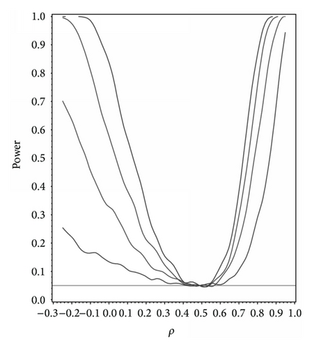
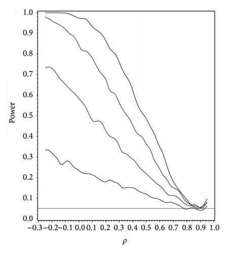
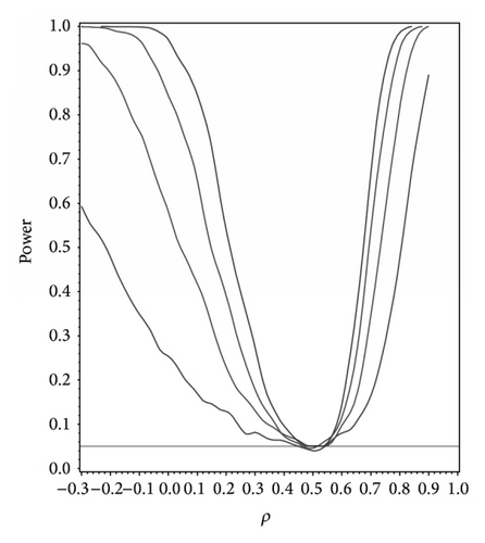
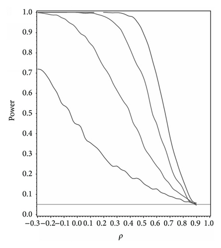
For the sake of example we modified our simulation and took ρ0 = 0.5 with marginals given by X1, X2 ~ N(0,1), , and X5exp(1, −1) with Γ0(ρ0) assumed to be compound symmetric under H0 and under H1. The results are shown in Figure 6 and as we can see they do not differ dramatically from Figure 2 assuming multivariate normality, thus illustrating the flexibility and nonparametric nature of our methodology.
As an additional result we studied the power under the correctly specified ρ under H0 with Γ0(ρ0) differing in structure. For this study we set ρ0 = 0.5,0.9 with Γ0(ρ0) set to compound symmetry under H0 and Γ0(ρ0) set to the first-order autoregressive structure under H1. In other words what is the power to detect a correlation structure different from the null structure given that ρ0 is the true correlation. At α = 0.05 the power to detect a different correlation structure under the alternative for ρ0 = 0.5 and 0.9 at n = 10,20,30,40 and α = 0.05 was 0.245, 0.539, 0.761, and 0.894 and 0.520, 0.858, 0.951, and 0.998, respectively.
4. Example
| Mouse | Day 0 | Day 1 | Day 2 | Day 3 | Day 4 |
|---|---|---|---|---|---|
| 1 | 21.4 | 21.0 | 21.0 | 21.3 | 21.5 |
| 2 | 18.4 | 18.4 | 18.0 | 18.1 | 17.8 |
| 3 | 17.8 | 17.6 | 17.4 | 17.2 | 17.1 |
| 4 | 18.2 | 18.5 | 17.6 | 18.0 | 17.5 |
| 5 | 20.0 | 19.4 | 19.1 | 19.6 | 18.9 |
| 6 | 20.2 | 19.3 | 19.3 | 19.3 | 18.6 |
| 7 | 16.5 | 16.3 | 16.6 | 16.4 | 16.3 |
| 8 | 17.6 | 17.4 | 17.5 | 17.9 | 17.6 |
| 9 | 19.8 | 20.4 | 20.1 | 20.6 | 20.3 |
| 10 | 22.0 | 22.3 | 21.3 | 21.9 | 20.7 |
| 11 | 17.5 | 17.4 | 17.5 | 17.5 | 17.3 |
| 12 | 20.3 | 20.2 | 19.8 | 20.4 | 19.7 |
| 13 | 16.3 | 16.2 | 16.2 | 15.9 | 15.7 |
| 14 | 18.0 | 17.2 | 17.2 | 17.0 | 16.4 |
| 15 | 20.3 | 19.9 | 19.0 | 18.9 | 18.1 |
| 16 | 21.4 | 21.2 | 20.7 | 21.1 | 20.7 |
| Day 0 | Day 1 | Day 2 | Day 3 | Day 4 | |
|---|---|---|---|---|---|
| Day 0 | 1.000 | 0.977 | 0.974 | 0.959 | 0.921 |
| Day 1 | 0.977 | 1.000 | 0.982 | 0.979 | 0.945 |
| Day 2 | 0.974 | 0.982 | 1.000 | 0.993 | 0.979 |
| Day 3 | 0.959 | 0.979 | 0.993 | 1.000 | 0.983 |
| Day 4 | 0.921 | 0.945 | 0.979 | 0.983 | 1.000 |
Given our overall P value from above which was 0.002, we may wish to examine in further detail what is driving us to reject H0. In this case we can examine specific submatrices of the dispersion matrix of . For this example we could test H0 : Σ = σΓ0(.95) using days 0, 1, and 2, only or any other combinations of days such that the appropriate correlation substructure is extracted from the original hypothesized values for Γ. For our example subtest we get P = 0.32 indicating no strong evidence against a first-order autoregressive “substructure” with equal variances and ρ0 = 0.95. If we add day 3, our P value = 0.04, indicating either the correlation structure may be misspecified at this point or the variance is different. Note that further work relative to the multiple comparison problem of subtests and their relative correlation is needed. This is simply an exploratory approach to this issue relative to the example at hand.
5. Concluding Remarks
In this note we provided a method for exact testing around specific covariance structures. We employed the Cholesky decomposition for this purpose. It was noted by a reviewer that other decomposition methodologies may lead to extensions of this methodology, which we will consider in terms of future work.
Conflict of Interests
The authors declare that there is no conflict of interests regarding the publication of this paper.
Acknowledgments
This research is supported by the NIH Grant 1R03DE020851-01A1, the National Institute of Dental and Craniofacial Research. The authors wish to thank the reviewers for their time and effort.


